Sometimes interpretability doesn’t cost predictive power

This was one of those times

Code in

Notetl;dr

A simple, interpretable model fit to features representing football concepts predicted as well as a neural network fit to player tracking data.

On this page

• The inspo
• The data
• The football features
• The model
• Did it cost predictive performance?
  • Can you believe the probabilities?
• What the model says
• The model on real plays
  • When the result is what the model expected
  • When the result is not what the model expected
  • Why the number moves
• The limits
• The wrap
• Appendix
  • Cross-validation
  • Chart and table helpers

The model’s estimated probability of a successful play, assuming the pass is caught (Broncos @ Giants, 2021 week 1). The rest of this post explains how that number gets made, and why it moves on this play.

The inspo

I came across a sports analytics project shared online in 2025 by Lou DiMuro that I really liked. It uses NFL player tracking data from the start of the 2021 and 2022 seasons to estimate, for plays where the QB throws a completed short pass, the probability the play will be successful. A short pass here is one where the receiver is at most 2 yards past the line of scrimmage when the ball is released. It has an awesome GIF showing the players’ movement as a play progresses with a live updating estimate (obviously inspired my video above). Very cool.

What counts as a ‘successful’ play in their analysis depends on the down:

• On 1st down, the play needs to gain ≥ 40% of the yards needed for a new set of downs
• On 2nd down, it needs to gain ≥ 60%
• On 3rd or 4th down, it needs to gain 100%

What’s interesting is that the model needs to account for the yards a receiver might gain after the catch, which aren’t known at the time of the pass. It’s judged on the outcome of the entire play (not just the pass). Only completed passes are included (no incompletions or interceptions), so it’s essentially asking “will the play gain enough yards assuming it’s caught?”

It uses a convolutional neural network (CNN) to estimate the probability of a successful play at the moment the ball is released. A strength of CNNs is that they can learn patterns from complex, high-dimensional inputs (e.g., position and velocity of all 22 players on the field). This comes at the cost of some interpretability. They can be very good at recognising situations that make a pass more or less likely to succeed, but understanding why the likelihood changes or how much different aspects of the play contribute to it is hard.

Whether interpretability like this matters depends on what we want from the model. If the main goal is pure prediction, giving a flexible model access to the full tracking data makes sense. But in applied sport environments, analysts also need to explain and discuss predictions with coaches or players who need to make decisions and actually do things in the game. Those conversations often turn to what might have happened if someone did something differently.

A coach wants to know:

If I ask a player to instead do it this way, what can I expect to change?

An athlete watching film might think:

If I do this, how might the defenders respond and how would that impact the play?

These are causal questions that can’t be answered from observational play data alone. What can be done though, is to represent the plays in football terms and examine how those representations relate to success. For example:

How does the space around a receiver at the time of the pass relate to the probability of a successful play?

How does the nearest defender’s closing speed relate to the chance of success?

Putting the questions in football terms like this gives coaches and players something concrete to challenge. They might disagree with how I’ve represented space or closing speed conceptually, or whether the relationships found make sense to them based on their domain knowledge. That discussion might uncover something worth testing with a research design that can estimate a causal effect.

My aim here is to turn the data used to train the CNN into a small set of domain-informed “football features” (e.g., space around a receiver, blocker positioning, etc) and use Bayesian logistic regression to model the probability of success. The features make my choices about how to represent the play explicit, the regression model makes the relationships easier to inspect, and the Bayesian approach lets me quantify and carry the uncertainty in those relationships through to the predicted probability of success.

The question is whether the transparency gained by making those football concepts explicit costs much in predictive performance.

The data

library(tidyverse)
library(cmdstanr)
library(posterior)
library(bayesplot)
library(ggdist)
library(patchwork)
library(ggtext)
library(gt)
library(SBC)

register_knitr_engine()
systemfonts::require_font("Poppins")

data_url <- "https://raw.githubusercontent.com/mitchhenderson/mitchhenderson.dev/main/posts/2026-10-19-nfl-interpretability-vs-predictive-power/data-public"

NotePython code outputs will differ from rendered results

The charts and tables on this page are made by the R code. The Python code runs the same analysis, but its charts are much simpler (no annotations or custom styling) and its tables use great_tables’ defaults. R and Python also use different random number generators and samplers (Stan through CmdStanR in R, PyMC in Python), so the exact numbers won’t match. The statistical results (the model’s estimates, the cross-validated scores and the probabilities) should be the same within the noise of random sampling.

import itertools
import math
import tempfile
import urllib.request

import arviz as az
import matplotlib.pyplot as plt
import numpy as np
import polars as pl
import pymc as pm
import rdata
import xarray as xr
from formulaic import model_matrix
from great_tables import GT
from scipy import stats
from scipy.special import expit

DATA_URL = "https://raw.githubusercontent.com/mitchhenderson/mitchhenderson.dev/main/posts/2026-10-19-nfl-interpretability-vs-predictive-power/data-public"

NAVY = "#134A8E"
PALE_NAVY = "#C4D2E3"
RED = "#E31937"

plt.rcParams.update({"axes.spines.top": False, "axes.spines.right": False})

The raw tracking data comes from the NFL’s Next Gen Stats Big Data Bowl. The data is available on Kaggle, split across two competitions. Big Data Bowl 2023 contains data from weeks 1–8 of the 2021 season and Big Data Bowl 2025 has weeks 1–9 of the 2022 season.

With ~50 frames per play and the position of every player and ball recorded at each frame, the full tracking dataset is ~3.7M rows. You can download it with a free Kaggle account after joining each competition and accepting the rules.

I didn’t work directly from the raw Kaggle data. I used the preprocessed data from Lou’s project GitHub repo, which captures only the completed short pass plays and transforms the data into tensors suitable for modelling with a neural network. It includes 3,228 plays, and 59% of them were successful. Instead of re-publishing the full 100+ MB dataset, I’ve included one play in the reference repo’s format as an example to demonstrate how I transformed it.

example_play <- read_rds(file.path(data_url, "example_play_tensor.rds"))

flatten_play_data <- function(tensors) {
  defender_rows <- expand_grid(
    play_row = seq_len(dim(tensors)[1]),
    defender_slot = seq_len(dim(tensors)[3])
  ) |>
    mutate(
      # The reference format stores each velocity as (y, x), not (x, y)
      defender_velocity_x = tensors[
        cbind(play_row, 2L, defender_slot, 1L)
      ],
      defender_velocity_y = tensors[
        cbind(play_row, 1L, defender_slot, 1L)
      ],
      defender_offset_downfield = tensors[cbind(
        play_row,
        3L,
        defender_slot,
        1L
      )],
      defender_offset_lateral = tensors[
        cbind(play_row, 4L, defender_slot, 1L)
      ],
      defender_velocity_relative_x = tensors[cbind(
        play_row,
        6L,
        defender_slot,
        1L
      )],
      defender_velocity_relative_y = tensors[cbind(
        play_row,
        5L,
        defender_slot,
        1L
      )]
    ) |>
    filter_out(defender_offset_downfield == 0, defender_offset_lateral == 0)

  blocker_rows <- expand_grid(
    play_row = seq_len(dim(tensors)[1]),
    defender_slot = seq_len(dim(tensors)[3]),
    offender_slot = seq_len(dim(tensors)[4])
  ) |>
    semi_join(defender_rows, by = join_by(play_row, defender_slot)) |>
    mutate(
      offender_offset_downfield = tensors[cbind(
        play_row,
        7L,
        defender_slot,
        offender_slot
      )],
      offender_offset_lateral = tensors[cbind(
        play_row,
        8L,
        defender_slot,
        offender_slot
      )],
      offender_velocity_relative_downfield = tensors[cbind(
        play_row,
        10L,
        defender_slot,
        offender_slot
      )],
      offender_velocity_relative_lateral = tensors[cbind(
        play_row,
        9L,
        defender_slot,
        offender_slot
      )]
    ) |>
    filter_out(offender_offset_downfield == 0, offender_offset_lateral == 0)

  play_context <- tibble(
    play_row = seq_len(dim(tensors)[1]),
    down = tensors[, 11L, 1L, 1L] * 3,
    yards_to_go = tensors[, 12L, 1L, 1L] * 29.5 + 0.5
  ) |>
    mutate(
      down = pmin(4L, pmax(1L, round(down))),
      # The yardage the play actually has to gain, given the down.
      yards_needed = recode_values(down, 1 ~ 0.4, 2 ~ 0.6, default = 1) *
        yards_to_go
    )

  list(
    defenders = defender_rows,
    blockers = blocker_rows,
    context = play_context
  )
}

tabular_play <- flatten_play_data(example_play)

def read_rds(url):
    """An array saved from R as .rds, and its attributes."""
    with tempfile.NamedTemporaryFile(suffix=".rds") as file:
        urllib.request.urlretrieve(url, file.name)
        parsed = rdata.parser.parse_file(file.name)
    converter = rdata.conversion.SimpleConverter()
    return converter.convert(parsed.object), converter.convert(parsed.object.attributes)


example_play, example_attributes = read_rds(f"{DATA_URL}/example_play_tensor.rds")


def flatten_play_data(tensors):
    n_plays, _, n_defenders, n_offence = tensors.shape

    def both_zero(prefix):
        return (pl.col(f"{prefix}_offset_downfield") == 0) & (
            pl.col(f"{prefix}_offset_lateral") == 0
        )

    play_row, defender_slot = np.meshgrid(
        np.arange(n_plays), np.arange(n_defenders), indexing="ij"
    )

    def defender(channel):
        return tensors[:, channel, :, 0].ravel()

    defender_rows = pl.DataFrame(
        {
            "play_row": play_row.ravel(),
            "defender_slot": defender_slot.ravel(),
            # The reference format stores each velocity as (y, x), not (x, y)
            "defender_velocity_x": defender(1),
            "defender_velocity_y": defender(0),
            "defender_offset_downfield": defender(2),
            "defender_offset_lateral": defender(3),
            "defender_velocity_relative_x": defender(5),
            "defender_velocity_relative_y": defender(4),
        }
    ).filter(~both_zero("defender"))

    play_row, defender_slot, offender_slot = np.meshgrid(
        np.arange(n_plays), np.arange(n_defenders), np.arange(n_offence), indexing="ij"
    )

    def offender(channel):
        return tensors[:, channel, :, :].ravel()

    blocker_rows = (
        pl.DataFrame(
            {
                "play_row": play_row.ravel(),
                "defender_slot": defender_slot.ravel(),
                "offender_slot": offender_slot.ravel(),
                "offender_offset_downfield": offender(6),
                "offender_offset_lateral": offender(7),
                "offender_velocity_relative_downfield": offender(9),
                "offender_velocity_relative_lateral": offender(8),
            }
        )
        .join(
            defender_rows.select("play_row", "defender_slot"),
            on=["play_row", "defender_slot"],
            how="semi",
        )
        .filter(~both_zero("offender"))
    )

    play_context = (
        pl.DataFrame(
            {
                "play_row": np.arange(n_plays),
                "down": tensors[:, 10, 0, 0] * 3,
                "yards_to_go": tensors[:, 11, 0, 0] * 29.5 + 0.5,
            }
        )
        .with_columns(down=pl.col("down").round().clip(1, 4).cast(pl.Int64))
        .with_columns(
            # The yardage the play actually has to gain, given the down
            yards_needed=pl.col("down").replace_strict({1: 0.4, 2: 0.6}, default=1.0)
            * pl.col("yards_to_go")
        )
    )

    return {
        "defenders": defender_rows,
        "blockers": blocker_rows,
        "context": play_context,
    }


tabular_play = flatten_play_data(example_play)

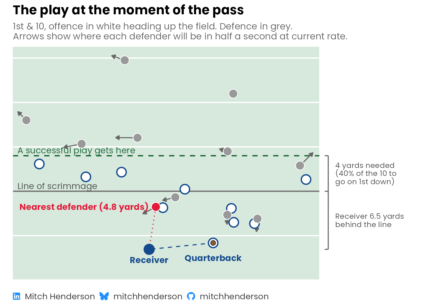
Here’s that play at the moment of release. Jacksonville Jaguars’ Trevor Lawrence passes to Jamal Agnew, who is 6.5 yards behind the line of scrimmage on 1st & 10 and gains 5. The reference format stores every player relative to the receiver, so Agnew is the fixed point everything is measured from.

dictionary <- read_csv(
  file.path(data_url, "feature_dictionary.csv"),
  show_col_types = FALSE
)

final_features <- dictionary |> pull(feature)

plays <- read_csv(
  file.path(data_url, "short_pass_features.csv"),
  show_col_types = FALSE
)

example_published <- plays |>
  filter(
    game_id == attr(example_play, "game_id"),
    play_id == attr(example_play, "play_id")
  )

plotted_defenders <- tabular_play |>
  pluck("defenders") |>
  mutate(
    distance = sqrt(defender_offset_downfield^2 + defender_offset_lateral^2),
    nearest = distance == min(distance)
  )

# Offensive players are stored relative to each defender, so one defender's
# copy is enough to place them
offence <- tabular_play$blockers |>
  slice_min(defender_slot, by = offender_slot) |>
  left_join(
    plotted_defenders |>
      select(defender_slot, defender_offset_downfield, defender_offset_lateral),
    by = join_by(defender_slot)
  ) |>
  mutate(
    lateral = defender_offset_lateral + offender_offset_lateral,
    downfield = defender_offset_downfield + offender_offset_downfield
  )

nearest_defender <- plotted_defenders |> filter(nearest)
line_of_scrimmage <- -example_published$receiver_depth
success_line <- line_of_scrimmage + example_published$yards_needed
field_edge <- min(plotted_defenders$defender_offset_lateral, offence$lateral) -
  1

# The brackets sit in a column to the right of the field
margin_x <- max(plotted_defenders$defender_offset_lateral, offence$lateral) +
  2.5

quarterback <- offence |> slice_min(downfield)

ordinal <- c("1st", "2nd", "3rd", "4th")

yards <- \(x) {
  x |>
    abs() |>
    scales::number(accuracy = 0.1, trim = TRUE) |>
    str_remove("\\.0$")
}

share_needed <- recode_values(
  example_published$down,
  1 ~ "40% of",
  2 ~ "60% of",
  c(3, 4) ~ "all of",
  unmatched = "error"
)

brackets <- tibble(
  bottom = c(0, line_of_scrimmage),
  top = c(line_of_scrimmage, success_line),
  label = c(
    str_glue(
      "Receiver {yards(line_of_scrimmage)} yards\nbehind the line"
    ),
    str_glue(
      "{yards(example_published$yards_needed)} yards needed\n({share_needed} the",
      " {example_published$yards_to_go} to\ngo on {ordinal[example_published$down]} down)"
    )
  )
)

field_green <- "#D7E8DC"
dark_green <- "#166534"

field <- tibble(
  xmin = field_edge - 0.5,
  xmax = margin_x - 1,
  ymin = min(offence$downfield, 0) - 3.5,
  ymax = max(plotted_defenders$defender_offset_downfield) + 1.5
)

yard_lines <- tibble(
  y = seq(line_of_scrimmage - 10, line_of_scrimmage + 25, by = 5)
) |>
  filter(y > field$ymin, y < field$ymax, y != line_of_scrimmage)

example_play_plot <- ggplot() +
  geom_rect(
    data = field,
    aes(xmin = xmin, xmax = xmax, ymin = ymin, ymax = ymax),
    fill = field_green
  ) +
  geom_segment(
    data = yard_lines,
    aes(x = field$xmin, xend = field$xmax, y = y, yend = y),
    colour = "white",
    linewidth = 0.8
  ) +
  annotate(
    "segment",
    x = field$xmin,
    xend = field$xmax,
    y = c(line_of_scrimmage, success_line),
    yend = c(line_of_scrimmage, success_line),
    colour = c("grey45", dark_green),
    linetype = c("solid", "dashed"),
    linewidth = 0.8
  ) +
  annotate(
    "text",
    x = field_edge,
    y = c(line_of_scrimmage, success_line) + 0.6,
    label = c("Line of scrimmage", "A successful play gets here"),
    colour = c("grey30", dark_green),
    family = "Poppins",
    size = 4,
    hjust = 0
  ) +
  geom_segment(
    data = plotted_defenders,
    aes(
      x = defender_offset_lateral,
      y = defender_offset_downfield,
      xend = defender_offset_lateral + defender_velocity_y / 2,
      yend = defender_offset_downfield + defender_velocity_x / 2
    ),
    colour = "grey40",
    arrow = arrow(length = unit(0.18, "cm"), type = "closed")
  ) +
  geom_segment(
    data = nearest_defender,
    aes(
      x = 0,
      y = 0,
      xend = defender_offset_lateral,
      yend = defender_offset_downfield
    ),
    colour = red,
    linetype = "dotted"
  ) +
  # As in the videos: the ball on the passer, tethered to the receiver
  annotate(
    "segment",
    x = quarterback$lateral,
    y = quarterback$downfield,
    xend = 0,
    yend = 0,
    colour = navy,
    linetype = "dashed"
  ) +
  geom_point(
    data = offence,
    aes(x = lateral, y = downfield),
    shape = 21,
    size = 5,
    stroke = 1.2,
    fill = "white",
    colour = navy
  ) +
  geom_point(
    data = plotted_defenders,
    aes(
      x = defender_offset_lateral,
      y = defender_offset_downfield,
      fill = nearest
    ),
    shape = 21,
    size = 5,
    colour = "white"
  ) +
  annotate("point", x = 0, y = 0, size = 6, colour = navy) +
  annotate(
    "point",
    x = quarterback$lateral,
    y = quarterback$downfield,
    shape = 21,
    size = 2.6,
    stroke = 0.6,
    colour = "grey20",
    fill = "#8a5a2b"
  ) +
  annotate(
    "text",
    x = c(
      0,
      quarterback$lateral,
      nearest_defender$defender_offset_lateral - 0.8
    ),
    y = c(
      -1.2,
      quarterback$downfield - 1.7,
      nearest_defender$defender_offset_downfield
    ),
    hjust = c(0.5, 0.5, 1),
    label = c(
      "Receiver",
      "Quarterback",
      str_glue("Nearest defender ({yards(nearest_defender$distance)} yards)")
    ),
    colour = c(navy, navy, red),
    family = "Poppins",
    fontface = "bold",
    size = 4,
    lineheight = 0.9
  ) +
  # Brackets for the two distances that matter most to the model, joined
  # where they meet at the line of scrimmage
  annotate(
    "segment",
    x = margin_x,
    xend = margin_x,
    y = 0,
    yend = success_line,
    colour = "grey40"
  ) +
  annotate(
    "segment",
    x = margin_x - 0.4,
    xend = margin_x,
    y = c(0, line_of_scrimmage, success_line),
    yend = c(0, line_of_scrimmage, success_line),
    colour = "grey40"
  ) +
  geom_text(
    data = brackets,
    aes(x = margin_x + 0.8, y = (bottom + top) / 2, label = label),
    hjust = 0,
    family = "Poppins",
    size = 3.5,
    lineheight = 0.9,
    colour = "grey30"
  ) +
  scale_fill_manual(
    values = c(`TRUE` = red, `FALSE` = "grey60"),
    guide = "none"
  ) +
  coord_equal(
    xlim = c(field$xmin, margin_x + 11),
    expand = FALSE,
    clip = "off"
  ) +
  labs(
    title = "The play at the moment of the pass",
    subtitle = str_glue(
      "{ordinal[example_published$down]} & {example_published$yards_to_go}, ",
      "offence in white heading up the field. Defence in grey.\n",
      "Arrows show where each defender will be in half a second at current rate."
    ),
    caption = socials
  ) +
  theme(
    axis.line = element_blank(),
    axis.text = element_blank(),
    axis.title.x = element_blank(),
    axis.title.y = element_blank(),
    plot.caption = element_markdown(hjust = 0)
  )

example_play_plot

dictionary = pl.read_csv(f"{DATA_URL}/feature_dictionary.csv")

final_features = dictionary["feature"].to_list()

plays = pl.read_csv(f"{DATA_URL}/short_pass_features.csv")

example_published = plays.filter(
    pl.col("game_id") == int(example_attributes["game_id"][0]),
    pl.col("play_id") == int(example_attributes["play_id"][0]),
)

plotted_defenders = (
    tabular_play["defenders"]
    .with_columns(
        distance=(
            pl.col("defender_offset_downfield") ** 2
            + pl.col("defender_offset_lateral") ** 2
        ).sqrt()
    )
    .with_columns(nearest=pl.col("distance") == pl.col("distance").min())
)

# Offensive players are stored relative to each defender, so one defender's
# copy is enough to place them
offence = (
    tabular_play["blockers"]
    .filter(
        pl.col("defender_slot") == pl.col("defender_slot").min().over("offender_slot")
    )
    .join(
        plotted_defenders.select(
            "defender_slot", "defender_offset_downfield", "defender_offset_lateral"
        ),
        on="defender_slot",
    )
    .with_columns(
        lateral=pl.col("defender_offset_lateral") + pl.col("offender_offset_lateral"),
        downfield=pl.col("defender_offset_downfield")
        + pl.col("offender_offset_downfield"),
    )
)

line_of_scrimmage = -example_published["receiver_depth"].item()
success_line = line_of_scrimmage + example_published["yards_needed"].item()

fig, ax = plt.subplots(figsize=(7, 6))
ax.axhline(line_of_scrimmage, color="grey", label="Line of scrimmage")
ax.axhline(
    success_line, color="green", linestyle="--", label="A successful play gets here"
)
# Where each defender will be in half a second at their current rate
ax.quiver(
    plotted_defenders["defender_offset_lateral"],
    plotted_defenders["defender_offset_downfield"],
    plotted_defenders["defender_velocity_y"] / 2,
    plotted_defenders["defender_velocity_x"] / 2,
    angles="xy",
    scale_units="xy",
    scale=1,
    width=0.004,
    color="grey",
)
ax.scatter(
    offence["lateral"], offence["downfield"], s=80, facecolor="white", edgecolor=NAVY
)
ax.scatter(
    plotted_defenders["defender_offset_lateral"],
    plotted_defenders["defender_offset_downfield"],
    s=80,
    color=np.where(plotted_defenders["nearest"], RED, "grey"),
)
ax.scatter(0, 0, s=100, color=NAVY, label="Receiver")
ax.set_aspect("equal")
ax.margins(0.08)
ax.set_xticks([])
ax.set_yticks([])
ax.legend(loc="upper center", bbox_to_anchor=(0.5, 0), ncol=3, frameon=False)
ax.set_title("The play at the moment of the pass")

The football features

With the tracking data in a simple tabular format, I can start creating features that describe the play in football terms. Instead of feeding the model every player’s position and velocity directly, I define things that I think might matter (e.g., how far the nearest defender is from the receiver and how quickly they’re closing that space).

The data says where the receiver and defenders are, but I’m deciding which football concepts within those measurements might inform the outcome. Someone with a different view of the game might choose differently. That’s a limitation, but it also puts the assumptions out in the open.

The simplest example is yards needed. The CNN was given the down and distance and had to learn the success rule from the data. I already know the rule, so I just calculated the yards each play needs and gave the model that instead.

The model I built uses nine features covering six concepts:

# The features for every play in a set of tables from flatten_play_data(),
# one row per play
# receiver_depth comes separately from the season play data, not the tensors.
# The line of scrimmage is at x = 60 after preprocessing, so receiver_depth
# is the receiver's x position at release minus 60 (positive beyond the line).
calculate_features <- function(tables) {
  defenders <- tables$defenders |>
    mutate(
      distance = sqrt(defender_offset_downfield^2 + defender_offset_lateral^2),
      # How fast the gap to the receiver is shrinking (positive is closing):
      # the relative velocity along the line between them
      closing_speed = -(defender_offset_downfield *
        defender_velocity_relative_x +
        defender_offset_lateral * defender_velocity_relative_y) /
        (distance + 1e-6)
    )

  around_the_receiver <- defenders |>
    summarise(
      # The nearest defender in front of the receiver, or the farthest
      # defender if nobody is in front
      space_ahead = if (any(defender_offset_downfield > 0)) {
        min(distance[defender_offset_downfield > 0])
      } else {
        max(distance)
      },
      room_beyond_nearest = space_ahead - min(distance),
      min_def_y_distance_to_rec = min(abs(defender_offset_lateral)),
      nearest_def_cushion = defender_offset_downfield[which.min(distance)],
      def_y_spread = sd(defender_offset_lateral),
      mean_top3_closing_speed = mean(head(closing_speed[order(distance)], 3)),
      nearest_defender = defender_slot[which.min(distance)],
      .by = play_row
    )

  # The nearest defender's closest offensive player, and their relative speed
  blockers <- tables$blockers |>
    inner_join(
      around_the_receiver |> select(play_row, defender_slot = nearest_defender),
      by = join_by(play_row, defender_slot)
    ) |>
    mutate(
      distance = sqrt(offender_offset_downfield^2 + offender_offset_lateral^2),
      relative_speed = sqrt(
        offender_velocity_relative_downfield^2 +
          offender_velocity_relative_lateral^2
      )
    ) |>
    summarise(
      nearest_blocker_advantage = min(distance),
      nearest_blocker_relative_speed = relative_speed[which.min(distance)],
      .by = play_row
    )

  tables$context |>
    select(play_row, yards_needed) |>
    left_join(
      around_the_receiver |> select(-space_ahead, -nearest_defender),
      by = join_by(play_row)
    ) |>
    left_join(blockers, by = join_by(play_row))
}

example_features <- calculate_features(tabular_play) |>
  pivot_longer(-play_row, names_to = "feature", values_to = "calculated") |>
  left_join(
    example_published |>
      select(all_of(setdiff(final_features, "receiver_depth"))) |>
      pivot_longer(everything(), names_to = "feature", values_to = "published"),
    by = join_by(feature)
  )

if (
  !isTRUE(all.equal(example_features$calculated, example_features$published))
) {
  cli::cli_abort("The features calculated here don't match the published ones.")
}

features_table <- dictionary |>
  select(group, label, description) |>
  gt(groupname_col = "group") |>
  post_table() |>
  cols_label(label = "Feature", description = "What it measures") |>
  cols_width(group ~ pct(19), label ~ pct(29)) |>
  tab_style(
    style = cell_text(weight = "600"),
    locations = cells_body(columns = label)
  ) |>
  tab_style(
    style = cell_text(color = "grey35", size = px(13)),
    locations = cells_body(columns = description)
  )

features_table

# The features for every play in a set of tables from flatten_play_data(),
# one row per play
# receiver_depth comes separately from the season play data, not the tensors.
# The line of scrimmage is at x = 60 after preprocessing, so receiver_depth
# is the receiver's x position at release minus 60 (positive beyond the line).
def calculate_features(tables):
    distance = (
        pl.col("defender_offset_downfield") ** 2
        + pl.col("defender_offset_lateral") ** 2
    ).sqrt()
    defenders = (
        tables["defenders"]
        .with_columns(distance=distance)
        .with_columns(
            # How fast the gap to the receiver is shrinking (positive is closing):
            # the relative velocity along the line between them
            closing_speed=-(
                pl.col("defender_offset_downfield")
                * pl.col("defender_velocity_relative_x")
                + pl.col("defender_offset_lateral")
                * pl.col("defender_velocity_relative_y")
            )
            / (pl.col("distance") + 1e-6)
        )
    )

    nearest = pl.col("distance").arg_min()
    in_front = pl.col("defender_offset_downfield") > 0
    around_the_receiver = (
        defenders.group_by("play_row")
        .agg(
            # The nearest defender in front of the receiver, or the farthest
            # defender if nobody is in front
            space_ahead=pl.when(in_front.any())
            .then(pl.col("distance").filter(in_front).min())
            .otherwise(pl.col("distance").max()),
            closest=pl.col("distance").min(),
            min_def_y_distance_to_rec=pl.col("defender_offset_lateral").abs().min(),
            nearest_def_cushion=pl.col("defender_offset_downfield").get(nearest),
            def_y_spread=pl.col("defender_offset_lateral").std(),
            mean_top3_closing_speed=pl.col("closing_speed")
            .sort_by("distance", maintain_order=True)
            .head(3)
            .mean(),
            nearest_defender=pl.col("defender_slot").get(nearest),
        )
        .with_columns(room_beyond_nearest=pl.col("space_ahead") - pl.col("closest"))
    )

    # The nearest defender's closest offensive player, and their relative speed
    blocker_distance = (
        pl.col("offender_offset_downfield") ** 2
        + pl.col("offender_offset_lateral") ** 2
    ).sqrt()
    blockers = (
        tables["blockers"]
        .join(
            around_the_receiver.select(
                "play_row", defender_slot=pl.col("nearest_defender")
            ),
            on=["play_row", "defender_slot"],
        )
        .with_columns(
            distance=blocker_distance,
            relative_speed=(
                pl.col("offender_velocity_relative_downfield") ** 2
                + pl.col("offender_velocity_relative_lateral") ** 2
            ).sqrt(),
        )
        .group_by("play_row")
        .agg(
            nearest_blocker_advantage=pl.col("distance").min(),
            nearest_blocker_relative_speed=pl.col("relative_speed").get(nearest),
        )
    )

    return (
        tables["context"]
        .select("play_row", "yards_needed")
        .join(
            around_the_receiver.drop("space_ahead", "closest", "nearest_defender"),
            on="play_row",
            how="left",
        )
        .join(blockers, on="play_row", how="left")
    )


example_features = calculate_features(tabular_play).drop("play_row")

if not np.allclose(
    example_features.to_numpy(),
    example_published.select(example_features.columns).to_numpy(),
):
    raise ValueError("The features calculated here don't match the published ones.")

GT(
    dictionary.select("group", "label", "description"), groupname_col="group"
).cols_label(label="Feature", description="What it measures")

	Feature	What it measures
What the play needs	Yards needed	The yardage the play has to gain to count as a success: 40% of the distance to the sticks on 1st down, 60% on 2nd, all of it on 3rd and 4th.
How deep the receiver is	Receiver depth	Where the receiver is relative to the line of scrimmage, in yards. Negative values mean the receiver is still behind it.
Space around the receiver	Extra room ahead	How much further away the nearest defender in front of the receiver is than the receiver's closest defender. Zero when the closest defender is the one in front.
	Closest defender across the field	Smallest sideline-to-sideline gap between the receiver and any defender.
	Nearest defender's cushion	How far downfield of the receiver the nearest defender is. Negative values mean the defender is trailing the receiver.
Shape of the defence	Defensive width	How spread out the defenders are across the field (standard deviation).
Who is arriving	Closing speed of the nearest three	Average closing speed of the three defenders closest to the receiver.
Help from blockers	Nearest defender's distance from a blocker	Distance from the closest defender to the nearest offensive player (which may be the quarterback). Larger values mean nobody is near enough to block that defender.
	Relative speed of the defender and nearest offensive player	How fast the closest defender and their nearest offensive player are moving relative to each other. Larger values mean their velocities differ more; they could be approaching or moving apart or across one another.
 Mitch Henderson  mitchhenderson  mitchhenderson

The model

Each play is either successful or it isn’t, so I’m modelling the probability of success with logistic regression. The model weights the features, adds their contributions to a baseline, and turns the total into a probability.

The model is written in the probabilistic programming languages Stan (run from R) and PyMC (Python).

// Logistic regression on standardised football features. Two of the
// features (yards needed and the nearest defender's cushion) arrive as natural
// spline columns, built in R, so their effect can bend.

data {
  int<lower=0> N;                    // plays the model learns from
  int<lower=1> K;                    // columns of the design matrix
  matrix[N, K] X;                    // standardised features and spline columns
  array[N] int<lower=0, upper=1> y;  // 1 = successful play

  int<lower=0> N_new;                // plays or frames to score
  matrix[N_new, K] X_new;

  int<lower=0, upper=1> prior_only;  // 1 = ignore the outcomes
}

parameters {
  real alpha;                        // log-odds of success for an average play
  vector[K] beta;                    // change in log-odds per standard deviation
}

model {
  alpha ~ normal(0, 1);
  beta ~ normal(0, 0.35);

  if (!prior_only) {
    y ~ bernoulli_logit_glm(X, alpha, beta);
  }
}

generated quantities {
  // Pointwise log-likelihood, for leave-one-out cross-validation
  vector[N] log_lik;
  // Outcomes the model would expect to see, for predictive checks
  array[N] int y_rep = bernoulli_logit_rng(alpha + X * beta);
  // Probability of success for the plays or frames being scored
  vector[N_new] p_new = inv_logit(alpha + X_new * beta);

  for (n in 1:N) {
    log_lik[n] = bernoulli_logit_lpmf(y[n] | alpha + X[n] * beta);
  }
}

# Logistic regression on standardised football features. Two of the
# features (yards needed and the nearest defender's cushion) arrive as natural
# spline columns (see the next chunk), so their effect can bend.
def build_model(X, y, X_new=None):
    X_new = X.clear() if X_new is None else X_new
    coords = {"column": X.columns, "play": range(X.height), "new": range(X_new.height)}

    with pm.Model(coords=coords) as model:
        # Log-odds of success for an average play
        alpha = pm.Normal("alpha", 0, 1)
        # Change in log-odds per standard deviation
        beta = pm.Normal("beta", 0, 0.35, dims="column")

        pm.Bernoulli(
            "y",
            logit_p=alpha + pm.math.dot(X.to_numpy(), beta),
            observed=y,
            dims="play",
        )
        # Probability of success for the plays or frames being scored
        pm.Deterministic(
            "p_new",
            pm.math.invlogit(alpha + pm.math.dot(X_new.to_numpy(), beta)),
            dims="new",
        )

    return model

The model assumes seven of the nine features have a straight-line relationship with the log odds of success. For the other two (yards needed and cushion), I let the model fit a curve (using splines). This is because going from 1 to 3 yards needed for a successful play is a big deal for a short pass, but 12 to 14 (same +2 yd difference) barely changes the odds (already low). When the nearest defender is close, an extra yard of space can be the difference between a tackle and a catch with room to run. When the defender’s already far away or behind the receiver, another yard doesn’t change much.

# Turn play-level features into the design matrix the Stan model is fitted on.
#
# Everything learned from the training plays (centres, scales and spline knots)
# is kept in a recipe and reused for any other plays or frames, so plays the
# model has not seen never inform their own preprocessing.

SPLINE_TERMS <- c(yards_needed = 4L, nearest_def_cushion = 3L)

design_recipe <- function(train, features, spline_terms = SPLINE_TERMS) {
  linear <- setdiff(features, names(spline_terms))
  bases <- imap(
    spline_terms,
    \(df, feature) splines::ns(train[[feature]], df = df)
  )

  list(
    linear = linear,
    centre = map_dbl(train[linear], mean),
    scale = map_dbl(train[linear], sd),
    bases = bases,
    curve_centre = map(bases, colMeans),
    curve_scale = map(bases, \(basis) map_dbl(as_tibble(basis), sd))
  )
}

design_matrix <- function(plays, recipe) {
  linear <- plays[recipe$linear] |>
    as.matrix() |>
    scale(center = recipe$centre, scale = recipe$scale)

  curves <- imap(recipe$bases, \(basis, feature) {
    curve <- predict(basis, plays[[feature]]) |>
      scale(
        center = recipe$curve_centre[[feature]],
        scale = recipe$curve_scale[[feature]]
      )
    colnames(curve) <- str_c(feature, "_curve", seq_len(ncol(curve)))
    curve
  })

  reduce(curves, cbind, .init = linear)
}

stan_data <- function(train, recipe, new = NULL, prior_only = FALSE) {
  X <- design_matrix(train, recipe)
  X_new <- if (is.null(new)) {
    X[0, , drop = FALSE]
  } else {
    design_matrix(new, recipe)
  }

  list(
    N = nrow(X),
    K = ncol(X),
    X = X,
    y = as.integer(train$success),
    N_new = nrow(X_new),
    X_new = X_new,
    prior_only = as.integer(prior_only)
  )
}

# Centres, scales and curve shapes are learned from the training plays
recipe <- design_recipe(plays, final_features)

# Turn play-level features into the design matrix the model is fitted on.
#
# Everything learned from the training plays (centres, scales and spline knots)
# is kept in a recipe and reused for any other plays or frames, so plays the
# model has not seen never inform their own preprocessing.

SPLINE_TERMS = {"yards_needed": 4, "nearest_def_cushion": 3}


def natural_spline(x, df):
    """A natural cubic spline for x, Python's usual stand-in for R's
    splines::ns(x, df). Centring the columns leaves the baseline to alpha."""
    spline = f"cr(x, df={df}, constraints='center') - 1"
    return model_matrix(spline, pl.DataFrame({"x": x})).model_spec


def spline_basis(spline, x):
    """The spline's columns at x. Beyond the outer knots the curve carries on
    as a straight line."""
    return np.asarray(spline.get_model_matrix(pl.DataFrame({"x": x})))


def design_recipe(train, features, spline_terms=SPLINE_TERMS):
    linear = [feature for feature in features if feature not in spline_terms]
    splines = {
        feature: natural_spline(train[feature], df)
        for feature, df in spline_terms.items()
    }
    curves = {
        feature: spline_basis(spline, train[feature])
        for feature, spline in splines.items()
    }

    return {
        "linear": linear,
        "centre": {feature: train[feature].mean() for feature in linear},
        "scale": {feature: train[feature].std() for feature in linear},
        "splines": splines,
        "curve_centre": {
            feature: curve.mean(axis=0) for feature, curve in curves.items()
        },
        "curve_scale": {
            feature: curve.std(axis=0, ddof=1) for feature, curve in curves.items()
        },
    }


def design_matrix(plays, recipe):
    linear = plays.select(
        (pl.col(feature) - recipe["centre"][feature]) / recipe["scale"][feature]
        for feature in recipe["linear"]
    )

    curves = []
    for feature, spline in recipe["splines"].items():
        curve = (
            spline_basis(spline, plays[feature]) - recipe["curve_centre"][feature]
        ) / (recipe["curve_scale"][feature])
        names = [f"{feature}_curve{i}" for i in range(1, curve.shape[1] + 1)]
        curves.append(pl.DataFrame(curve, schema=names, orient="row"))

    return pl.concat([linear, *curves], how="horizontal")


# Centres, scales and curve shapes are learned from the training plays
recipe = design_recipe(plays, final_features)

# The training plays as the model sees them
X = design_matrix(plays, recipe)
y = plays["success"].to_numpy()

NotePrior predictive check and simulation-based calibration (technical details)

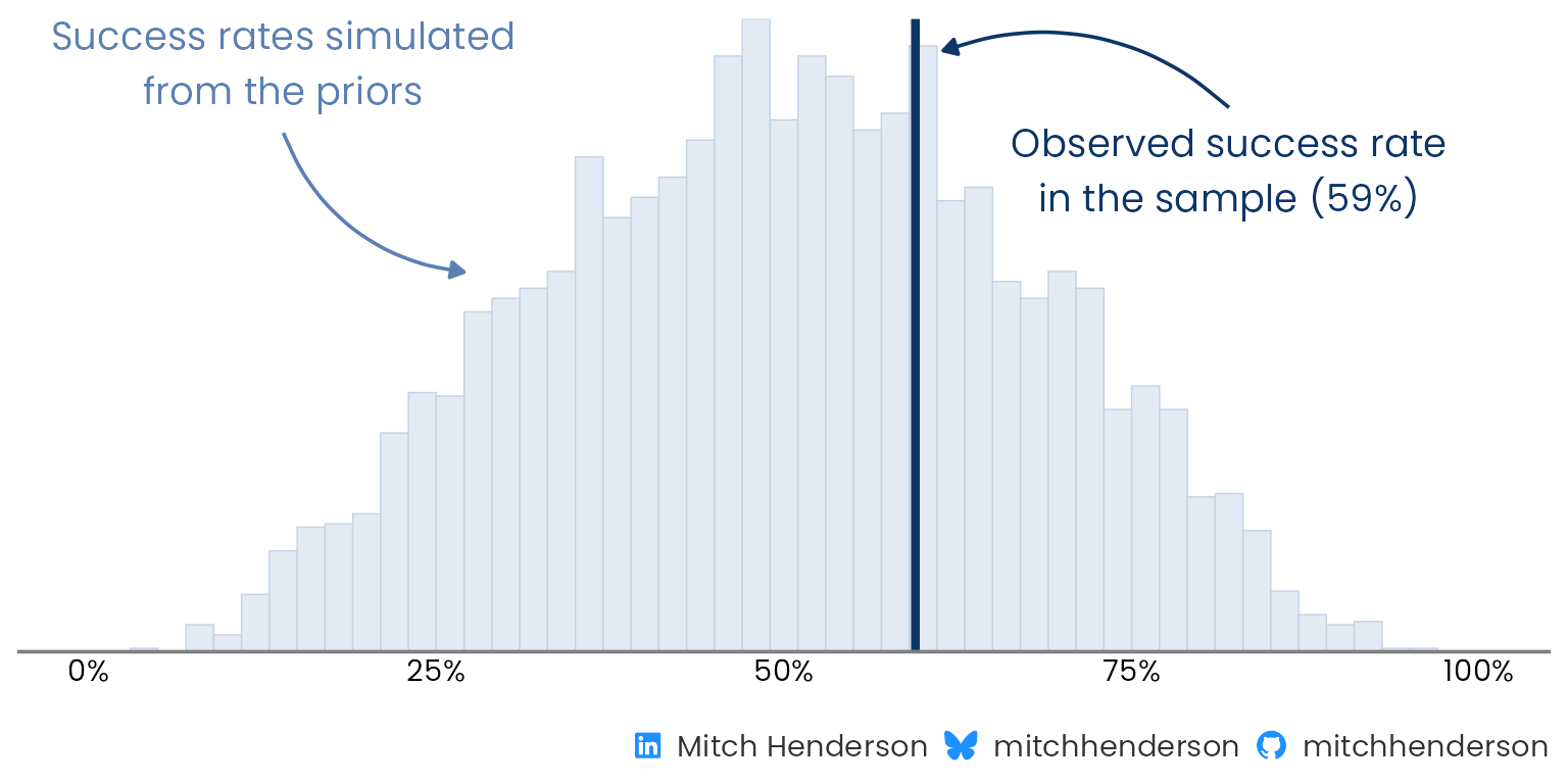
Do the priors make sense? Bayesian models like this one need priors representing our beliefs about the distribution of plausible parameter values. Because thinking about parameters and understanding their impact on observed outcomes isn’t natural to most psychologically well-adjusted humans, it’s good practice to simulate outcome data using parameter values drawn from our prior distributions. This way we can see if those choices of priors generate outcome values within the realms of reality.

In this case, the priors allow a wide range of plausible success rates (about 20–80%) that comfortably includes the observed 59%.

prior_fit <- model$sample(
  data = stan_data(plays, recipe, prior_only = TRUE),
  seed = 2534,
  chains = 4,
  parallel_chains = 4,
  iter_warmup = 1000,
  iter_sampling = 1000,
  refresh = 0
)

prior_check <- ppc_stat(
  y = plays$success,
  yrep = prior_fit$draws("y_rep", format = "matrix"),
  stat = "mean",
  binwidth = 0.02
)

# Annotations sit relative to the tallest bar
tallest_bar <- max(layer_data(prior_check, 1)$count)
observed <- mean(plays$success)
simulated_blue <- "#5B80B3"
observed_blue <- "#0D3566"

prior_check_plot <- prior_check +
  annotate(
    "curve",
    x = 0.14,
    xend = 0.27,
    y = 0.82 * tallest_bar,
    yend = 0.6 * tallest_bar,
    curvature = 0.3,
    arrow = arrow(length = unit(2, "mm"), type = "closed"),
    colour = simulated_blue
  ) +
  annotate(
    "text",
    x = 0.14,
    y = 0.93 * tallest_bar,
    label = "Success rates simulated\nfrom the priors",
    hjust = 0.5,
    colour = simulated_blue,
    family = "Poppins"
  ) +
  annotate(
    "curve",
    x = 0.82,
    xend = observed + 0.02,
    y = 0.86 * tallest_bar,
    yend = 0.95 * tallest_bar,
    curvature = 0.3,
    arrow = arrow(length = unit(2, "mm"), type = "closed"),
    colour = observed_blue
  ) +
  annotate(
    "text",
    x = 0.82,
    y = 0.76 * tallest_bar,
    label = str_glue(
      "Observed success rate\nin the sample ({scales::percent(observed, accuracy = 1)})"
    ),
    hjust = 0.5,
    colour = observed_blue,
    family = "Poppins"
  ) +
  scale_x_continuous(labels = scales::label_percent(), limits = c(0, 1)) +
  labs(
    x = NULL,
    caption = socials
  ) +
  theme(
    legend.position = "none",
    axis.line.y = element_blank(),
    axis.text.y = element_blank()
  )

prior_check_plot

with build_model(X, y):
    prior = pm.sample_prior_predictive(draws=4000, random_seed=2534)

# The overall success rate in each dataset simulated from the priors
prior_rates = prior.prior_predictive["y"].mean("play").values.ravel()

fig, ax = plt.subplots(figsize=(8, 4))
ax.hist(prior_rates, bins=np.arange(0, 1.02, 0.02), color=PALE_NAVY)
ax.axvline(y.mean(), color=NAVY)
ax.set_xlim(0, 1)
ax.set_yticks([])
ax.set_xlabel("Success rate (line: observed)")

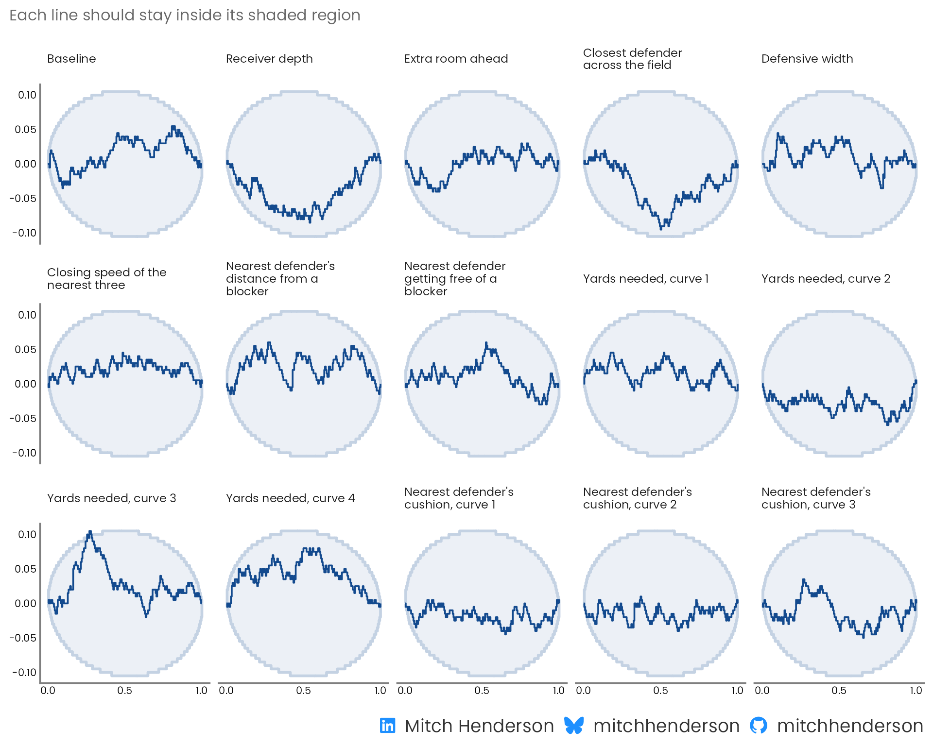
Can the model recover known parameter values? The prior predictive check above looks at whether the priors are sensible, but doesn’t validate that the model can find true parameter values. If I simulate data using known parameters drawn from the priors and fit the model to the simulated data, do the model’s estimates line up with the true values? Does each true value land in the middle half of the model’s estimates about half the time, in the top tenth about a tenth of the time, etc? Simulation-based calibration checks this by fitting the model 200 times on different randomly simulated datasets. Because it’s fitting the model 200 times, this part is computationally expensive (i.e., slow: about 15–20 min on my M5 MacBook Air).

In the chart below, each panel is one parameter. All but one of the lines stay inside the shaded bands (the third yards-needed curve pokes outside). The shaded regions are the area the line should stay in 95% of the time if the fitting works, so with 15 parameters one just poking out isn’t a concern.

sbc_data <- stan_data(plays, recipe)

# One simulated dataset: parameters drawn from the priors, then an outcome for
# every real play from those parameters
simulate_dataset <- function(data) {
  alpha <- rnorm(1, 0, 1)
  beta <- rnorm(data$K, 0, 0.35)
  log_odds <- alpha + drop(data$X %*% beta)

  list(
    variables = list(alpha = alpha, beta = beta),
    generated = modifyList(
      data,
      list(y = rbinom(data$N, 1, plogis(log_odds)))
    )
  )
}

set.seed(20261007)
datasets <- generate_datasets(
  SBC_generator_function(simulate_dataset, data = sbc_data),
  n_sims = 200
)

# The same sampler settings as the real fit, four simulations at a time
backend <- SBC_backend_cmdstan_sample(
  model,
  chains = 4,
  iter_warmup = 1000,
  iter_sampling = 1000
)

future::plan(future::multisession, workers = 4)
sbc <- compute_SBC(datasets, backend, keep_fits = FALSE)
future::plan(future::sequential)

# Name each weight after its feature (a curve has several weights)
weight_names <- tibble(
  variable = c("alpha", str_glue("beta[{seq_len(sbc_data$K)}]")),
  column = c("intercept", colnames(sbc_data$X))
) |>
  mutate(
    feature = str_remove(column, "_curve\\d+$"),
    curve = str_extract(column, "(?<=_curve)\\d+")
  ) |>
  left_join(dictionary |> select(feature, label), by = join_by(feature)) |>
  mutate(
    name = case_when(
      column == "intercept" ~ "Baseline",
      !is.na(curve) ~ str_glue("{label}, curve {curve}"),
      .default = label
    )
  )
weight_order <- str_wrap(weight_names$name, 22)

sbc$stats |>
  mutate(
    variable = recode_values(
      variable,
      from = weight_names$variable,
      to = weight_names$name,
      unmatched = "error"
    ) |>
      str_wrap(22)
  ) |>
  plot_ecdf_diff() +
  # The post's colours, and the weights in the order of the feature table
  scale_colour_manual(
    values = c(`theoretical CDF` = pale_navy, `sample ECDF` = navy),
    guide = "none"
  ) +
  scale_fill_manual(
    values = c(`theoretical CDF` = pale_navy, `sample ECDF` = "transparent"),
    guide = "none"
  ) +
  facet_wrap(vars(factor(group, levels = weight_order)), ncol = 5) +
  scale_x_continuous(breaks = c(0, 0.5, 1)) +
  labs(
    subtitle = "Each line should stay inside its shaded region",
    caption = socials
  ) +
  theme(
    strip.text = element_text(size = 9, face = "plain", lineheight = 0.9),
    axis.text = element_text(size = 8)
  )

rng = np.random.default_rng(20261007)
n_sims = 200
X_matrix = X.to_numpy()


# One simulated dataset: parameters drawn from the priors, then an outcome for
# every real play from those parameters
def simulate_dataset(rng):
    alpha = rng.normal(0, 1)
    beta = rng.normal(0, 0.35, X.width)
    log_odds = alpha + X_matrix @ beta
    return np.r_[alpha, beta], rng.binomial(1, expit(log_odds))


ranks, divergences, rhats = [], [], []
for _ in range(n_sims):
    truth, simulated_y = simulate_dataset(rng)
    # The same sampler settings as the real fit
    with build_model(X, simulated_y):
        sbc_fit = pm.sample(
            1000, tune=1000, chains=4, random_seed=rng, progressbar=False
        )

    posterior = sbc_fit.posterior
    draws = np.column_stack(
        [
            posterior["alpha"].values.ravel(),
            posterior["beta"].values.reshape(-1, X.width),
        ]
    )
    # Where each true value ranks among the draws, thinned to every 10th draw
    # so the ranks aren't distorted by autocorrelation
    ranks.append((draws[::10] < truth).mean(axis=0))
    divergences.append(int(sbc_fit.sample_stats["diverging"].sum()))
    convergence = az.summary(sbc_fit, var_names=["alpha", "beta"], kind="diagnostics")
    rhats.append(convergence["r_hat"].max())

pit = xr.Dataset(
    {"pit": (("chain", "draw", "parameter"), np.array(ranks)[None])},
    coords={"parameter": ["alpha", *X.columns]},
)
az.plot_ecdf_pit(xr.DataTree.from_dict({"prior_sbc": pit}))

print(
    f"{sum(divergences)} divergent transitions across {n_sims} simulated datasets; "
    f"largest R-hat {max(rhats):.3f}"
)

Across the 200 simulated datasets there were 0 divergent transitions, and the largest R-hat was 1.008.

Then I fit it to all 3,228 plays.

NoteFitting the model and checking the sampler (technical details)

frames <- read_csv(
  file.path(data_url, "withheld_play_frames.csv"),
  show_col_types = FALSE
)

fit <- model$sample(
  data = stan_data(plays, recipe, new = frames),
  seed = 2534,
  chains = 4,
  parallel_chains = 4,
  iter_warmup = 1000,
  iter_sampling = 1000,
  refresh = 0
)

# Every plausible set of weights, kept together as random variables
draws <- as_draws_rvars(fit$draws(c("alpha", "beta")))

inv_logit <- \(log_odds) 1 / (1 + exp(-log_odds))

predict_success <- function(plays) {
  log_odds <- draws$alpha +
    drop(
      design_matrix(plays, recipe) %**% draws$beta
    )
  inv_logit(log_odds)
}

# Yards needed is a whole number in the first frames, so the column types are
# read from the whole file
frames = pl.read_csv(f"{DATA_URL}/withheld_play_frames.csv", infer_schema_length=None)

with build_model(X, y, design_matrix(frames, recipe)) as model:
    fit = pm.sample(1000, tune=1000, chains=4, random_seed=2534)
    # Pointwise log-likelihood, for leave-one-out cross-validation
    pm.compute_log_likelihood(fit)

# Every plausible set of weights: one row per posterior draw
alpha_draws = fit.posterior["alpha"].values.ravel()
beta_draws = fit.posterior["beta"].values.reshape(-1, X.width)


def predict_success(plays):
    """The probability of success for each play (columns), for every draw (rows)."""
    log_odds = (
        alpha_draws[:, None] + beta_draws @ design_matrix(plays, recipe).to_numpy().T
    )
    return expit(log_odds)

Did the fitting work? Yes. These are the standard checks that the sampler explored properly, and that no single play pulls too hard on the fit.

sampler <- fit$diagnostic_summary(quiet = TRUE)
# How much any one play pulls on the fit, from leave-one-out cross-validation
pareto_k <- fit$loo()$diagnostics$pareto_k
convergence <- fit$draws(c("alpha", "beta")) |>
  summarise_draws(rhat, ess_bulk, ess_tail)

passed <- pill("Pass", "#166534", "#DCFCE7")
failed <- pill("Fail", "#B4122B", "#FCE4E8")

diagnostics_table <- tribble(
  ~check                                 , ~value                         , ~want        , ~ok                                 ,
  "Largest R-hat"                        , max(convergence$rhat)          , "Below 1.01" , max(convergence$rhat) < 1.01        ,
  "Smallest effective sample size, bulk" , min(convergence$ess_bulk)      , "Above 400"  , min(convergence$ess_bulk) > 400     ,
  "Smallest effective sample size, tail" , min(convergence$ess_tail)      , "Above 400"  , min(convergence$ess_tail) > 400     ,
  "Divergent transitions"                , sum(sampler$num_divergent)     , "0"          , sum(sampler$num_divergent) == 0     ,
  "Maximum tree depth reached"           , sum(sampler$num_max_treedepth) , "0"          , sum(sampler$num_max_treedepth) == 0 ,
  "Lowest E-BFMI"                        , min(sampler$ebfmi)             , "Above 0.3"  , min(sampler$ebfmi) > 0.3            ,
  "Largest Pareto k, leave-one-out"      , max(pareto_k)                  , "Below 0.7"  , max(pareto_k) < 0.7
) |>
  mutate(ok = if_else(ok, passed, failed)) |>
  gt() |>
  post_table() |>
  fmt_number(columns = value, decimals = 0) |>
  fmt_number(columns = value, rows = check == "Largest R-hat", decimals = 3) |>
  fmt_number(
    columns = value,
    rows = check %in% c("Lowest E-BFMI", "Largest Pareto k, leave-one-out"),
    decimals = 2
  ) |>
  fmt_markdown(columns = ok) |>
  cols_label(
    check = "Check",
    value = "This model",
    want = "What I want to see",
    ok = ""
  ) |>
  tab_style(
    style = cell_text(weight = "600"),
    locations = cells_body(columns = value)
  ) |>
  tab_style(
    style = cell_text(color = "grey40"),
    locations = cells_body(columns = want)
  )

diagnostics_table

convergence = az.summary(fit, var_names=["alpha", "beta"], kind="diagnostics")
# How much any one play pulls on the fit, from leave-one-out cross-validation
pareto_k = az.loo(fit, pointwise=True).pareto_k.values

# Each check: (this model's value, what I want to see, whether it passes)
results = {
    "Largest R-hat": (convergence["r_hat"].max(), "Below 1.01", lambda v: v < 1.01),
    "Smallest effective sample size, bulk": (
        convergence["ess_bulk"].min(),
        "Above 400",
        lambda v: v > 400,
    ),
    "Smallest effective sample size, tail": (
        convergence["ess_tail"].min(),
        "Above 400",
        lambda v: v > 400,
    ),
    "Divergent transitions": (
        fit.sample_stats["diverging"].sum().item(),
        "0",
        lambda v: v == 0,
    ),
    "Maximum tree depth reached": (
        fit.sample_stats["reached_max_treedepth"].sum().item(),
        "0",
        lambda v: v == 0,
    ),
    "Lowest E-BFMI": (
        az.bfmi(fit)["energy"].min().item(),
        "Above 0.3",
        lambda v: v > 0.3,
    ),
    "Largest Pareto k, leave-one-out": (pareto_k.max(), "Below 0.7", lambda v: v < 0.7),
}

checks = pl.DataFrame(
    [
        {
            "check": check,
            "value": float(value),
            "want": want,
            "ok": "Pass" if passes(value) else "Fail",
        }
        for check, (value, want, passes) in results.items()
    ]
)

(
    GT(checks)
    .fmt_number(columns="value", decimals=0)
    .fmt_number(columns="value", rows=[0], decimals=3)
    .fmt_number(columns="value", rows=[5, 6], decimals=2)
    .cols_label(check="Check", value="This model", want="What I want to see", ok="")
)

Check	This model	What I want to see
Largest R-hat	1.003	Below 1.01	Pass
Smallest effective sample size, bulk	3,584	Above 400	Pass
Smallest effective sample size, tail	2,578	Above 400	Pass
Divergent transitions	0	0	Pass
Maximum tree depth reached	0	0	Pass
Lowest E-BFMI	0.91	Above 0.3	Pass
Largest Pareto k, leave-one-out	0.27	Below 0.7	Pass
 Mitch Henderson  mitchhenderson  mitchhenderson

NotePosterior predictive check (technical details)

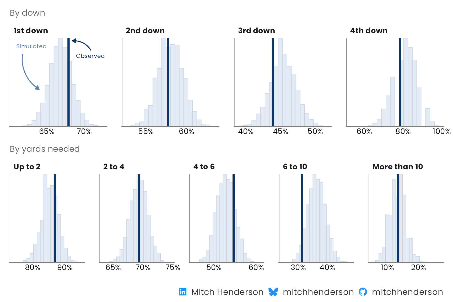
If the model is a good (albeit simplified) representation of reality, the outcomes it simulates should look like the ones observed in the real world. And they should do this across different subsets of interest (to show it’s not just good in some areas but not others).

Here I use the model to simulate outcomes for every play in the training data, then compare the distribution of the simulated success rates with the actual success rates across downs and across yards needed for success. The observed rate is inside the model’s expected plausible range in each scenario. The weakest spot is on plays needing 6 to 10 yards, where the model is a bit optimistic.

y_rep <- fit$draws("y_rep", format = "matrix")

check_by <- function(group, title) {
  ppc_stat_grouped(
    y = plays$success,
    yrep = y_rep,
    group = group,
    stat = "mean",
    facet_args = list(nrow = 1),
    bins = 20
  ) +
    scale_x_continuous(
      labels = scales::label_percent(accuracy = 1),
      breaks = scales::breaks_pretty(n = 2)
    ) +
    labs(subtitle = title, x = NULL) +
    theme(
      legend.position = "none",
      axis.line.y = element_blank(),
      axis.text.y = element_blank(),
      axis.text.x = element_text(size = 11),
      panel.spacing.x = unit(1.5, "lines")
    )
}

plays_by_down <- recode_values(
  plays$down,
  1 ~ "1st down",
  2 ~ "2nd down",
  3 ~ "3rd down",
  4 ~ "4th down"
)

by_down <- check_by(plays_by_down, "By down")

# Labels on the first panel say which mark is which. They stay below the
# tallest bar so the panel keeps its scale
first_down <- plays$down == 1
first_down_rates <- rowMeans(y_rep[, first_down])
first_down_observed <- mean(plays$success[first_down])
first_down_peak <- layer_data(by_down, 1) |>
  filter(PANEL == 1) |>
  pull(count) |>
  max()
first_panel <- \(...) {
  tibble(
    group = factor("1st down", levels = levels(factor(plays_by_down))),
    ...
  )
}

by_down <- by_down +
  geom_curve(
    data = first_panel(
      x = min(first_down_rates) + 0.008,
      xend = quantile(first_down_rates, 0.03),
      y = 0.82 * first_down_peak,
      yend = 0.42 * first_down_peak
    ),
    aes(x = x, y = y, xend = xend, yend = yend),
    curvature = 0.3,
    arrow = arrow(length = unit(2, "mm"), type = "closed"),
    colour = simulated_blue,
    inherit.aes = FALSE
  ) +
  geom_text(
    data = first_panel(
      x = min(first_down_rates),
      y = 0.91 * first_down_peak,
      label = "Simulated"
    ),
    aes(x = x, y = y, label = label),
    hjust = 0,
    size = 3,
    colour = simulated_blue,
    family = "Poppins",
    inherit.aes = FALSE
  ) +
  geom_curve(
    data = first_panel(
      x = first_down_observed + 0.03,
      xend = first_down_observed + 0.005,
      y = 0.86 * first_down_peak,
      yend = 0.97 * first_down_peak
    ),
    aes(x = x, y = y, xend = xend, yend = yend),
    curvature = 0.3,
    arrow = arrow(length = unit(2, "mm"), type = "closed"),
    colour = observed_blue,
    inherit.aes = FALSE
  ) +
  geom_text(
    data = first_panel(
      x = first_down_observed + 0.01,
      y = 0.8 * first_down_peak,
      label = "Observed"
    ),
    aes(x = x, y = y, label = label),
    hjust = 0,
    size = 3,
    colour = observed_blue,
    family = "Poppins",
    inherit.aes = FALSE
  )

by_yards_needed <- check_by(
  cut(
    plays$yards_needed,
    breaks = c(0, 2, 4, 6, 10, Inf),
    labels = c("Up to 2", "2 to 4", "4 to 6", "6 to 10", "More than 10")
  ),
  "By yards needed"
)

posterior_check_plot <- by_down /
  by_yards_needed +
  plot_annotation(
    caption = socials
  )

posterior_check_plot

with model:
    posterior_predictive = pm.sample_posterior_predictive(fit, random_seed=2534)

y_rep = posterior_predictive.posterior_predictive["y"].values.reshape(-1, X.height)

down_labels = ["1st down", "2nd down", "3rd down", "4th down"]
by_down = plays["down"].replace_strict(dict(enumerate(down_labels, start=1)))

yards_labels = ["Up to 2", "2 to 4", "4 to 6", "6 to 10", "More than 10"]
by_yards_needed = (
    plays["yards_needed"].cut([2, 4, 6, 10], labels=yards_labels).cast(pl.String)
)

# The success rate in each simulated dataset against the observed rate, for
# every group of plays
fig, axes = plt.subplots(2, 5, figsize=(12, 5))
for row, groups, labels in zip(
    axes, [by_down, by_yards_needed], [down_labels, yards_labels]
):
    for ax, label in zip(row, labels):
        in_group = (groups == label).to_numpy()
        ax.hist(y_rep[:, in_group].mean(axis=1), bins=20, color=PALE_NAVY)
        ax.axvline(y[in_group].mean(), color=NAVY)
        ax.set_title(label, loc="left", fontsize=10)
        ax.set_yticks([])
axes[0, -1].axis("off")
fig.tight_layout()

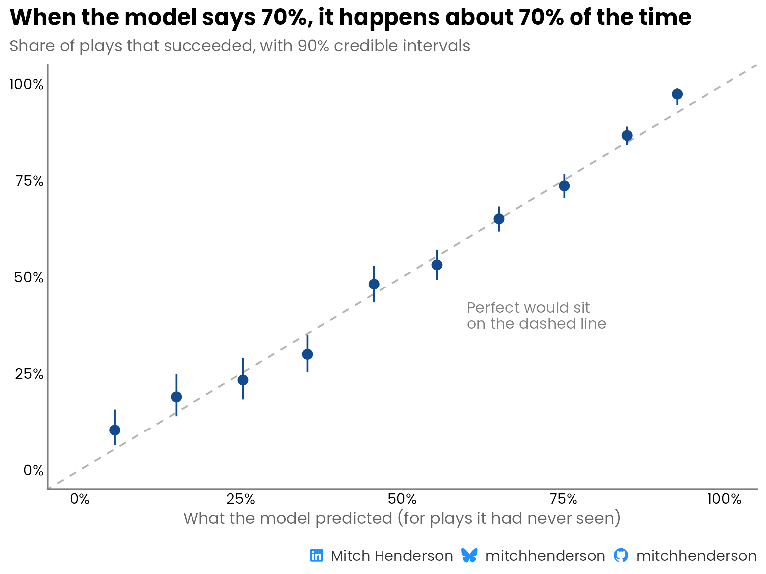
The posterior predictive check shows that the model is able to accurately recover observed success rates across downs and across yards needed, but that’s on plays the model has already seen. Its probabilities need to hold up on plays it hasn’t seen to be practically useful.

Did it cost predictive performance?

Did making the football concepts explicit and using a simpler, interpretable model cost much in predictive performance? No. 

It performed as well as the CNN, and a little better on every metric the CNN reports.

To make the comparison as fair as I could, I copied the reference eval by using the same 3,228 plays, the same five-fold cross-validation approach (stratified, seed 42), and the same definition of each metric.¹ That’s only possible because Lou published the plays, how they were split, and exactly how the model’s performance was assessed 🙌 (many don’t do this). Every prediction here was made by a version of the model that never saw that play (the code that does this is in the appendix).

# Area under the precision-recall curve by the trapezoid rule, with an anchor
# at (recall 0, precision 1). This is sklearn's auc(recall, precision), the
# definition the reference CNN reports, and it gives a slightly different
# number from the step-wise "average precision".
pr_auc_trapz <- function(prob, y) {
  n_pos <- sum(y == 1L)
  if (n_pos == 0L || n_pos == length(y)) {
    return(NA_real_)
  }
  # A threshold includes every play with the same predicted probability.
  thresholds <- tibble(prob, y) |>
    summarise(n = n(), successes = sum(y == 1L), .by = prob) |>
    arrange(desc(prob)) |>
    mutate(
      true_positives = cumsum(successes),
      predicted_positives = cumsum(n)
    )
  precision <- c(1, thresholds$true_positives / thresholds$predicted_positives)
  recall <- c(0, thresholds$true_positives / n_pos)
  sum(diff(recall) * (precision[-length(precision)] + precision[-1]) / 2)
}

# Area under the ROC curve from the rank-sum identity.
roc_auc_fast <- function(prob, y) {
  n_pos <- sum(y == 1L)
  n_neg <- sum(y == 0L)
  if (n_pos == 0L || n_neg == 0L) {
    return(NA_real_)
  }
  ranks <- rank(prob, ties.method = "average")
  (sum(ranks[y == 1L]) - n_pos * (n_pos + 1) / 2) / (n_pos * n_neg)
}

# The four metrics the reference CNN reports, as a one-row tibble.
performance <- function(prob, y) {
  tibble(
    pr_auc = pr_auc_trapz(prob, y),
    roc_auc = roc_auc_fast(prob, y),
    accuracy = mean((prob >= 0.5) == (y == 1L)),
    brier = mean((prob - y)^2)
  )
}

# Predicted probabilities in equal-width bins against how often those plays
# succeeded. `lower` and `upper` are a 90% interval on the observed rate.
calibration_data <- function(prob_mean, y, n_bins = 10) {
  tibble(prob_mean = prob_mean, y = y) |>
    mutate(
      bin = cut(
        prob_mean,
        breaks = seq(0, 1, length.out = n_bins + 1),
        include.lowest = TRUE,
        labels = FALSE
      )
    ) |>
    summarise(
      n = n(),
      n_success = sum(y),
      mean_pred = mean(prob_mean),
      mean_obs = mean(y),
      lower = qbeta(0.05, n_success + 0.5, n - n_success + 0.5),
      upper = qbeta(0.95, n_success + 0.5, n - n_success + 0.5),
      .by = bin
    ) |>
    arrange(bin)
}

# `reference` holds the cross-validated predictions (the code is in the
# appendix)

model_performance <- performance(reference$p_mean, reference$success)

success_rate <- mean(reference$success)

comparison <- bind_rows(
  # Conventional no-skill PR reference; constant mean predictions for the
  # accuracy and Brier baselines
  tibble(
    model = "No-skill baseline",
    detail = "No tracking features",
    pr_auc = success_rate,
    roc_auc = 0.5,
    accuracy = mean((success_rate >= 0.5) == (reference$success == 1L)),
    brier = mean((success_rate - reference$success)^2)
  ),
  # Published by the reference project, averaged over four training runs
  tibble(
    model = "Reference CNN",
    detail = "Published neural network",
    pr_auc = 0.7929,
    roc_auc = 0.7314,
    accuracy = 0.6808,
    brier = 0.2026
  ),
  model_performance |>
    mutate(
      model = "This model",
      detail = "Bayesian logistic regression on nine football features"
    )
)

comparison_table <- comparison |>
  mutate(
    model = str_glue(
      "<div style='font-weight:600;'>{model}</div>",
      "<div style='font-size:12px; color:#666666;'>{detail}</div>"
    )
  ) |>
  select(-detail) |>
  gt() |>
  post_table(
    note = "* Lower is better. Higher is better for the other scores."
  ) |>
  fmt_markdown(columns = model) |>
  fmt_number(columns = -model, decimals = 3) |>
  cols_label(
    model = "",
    pr_auc = "PR-AUC",
    roc_auc = "ROC-AUC",
    accuracy = "Accuracy",
    brier = "Brier score*"
  ) |>
  cols_align(align = "left", columns = model) |>
  cols_align(align = "right", columns = -model) |>
  tab_style(
    style = cell_fill("#EEF3F9"),
    locations = cells_body(rows = 3)
  )

comparison_table

def pr_auc_trapz(prob, y):
    """Area under the precision-recall curve by the trapezoid rule.

    Anchored at (recall 0, precision 1). This is sklearn's auc(recall, precision),
    the definition the reference CNN reports, and it gives a slightly different
    number from the step-wise "average precision".
    """
    n_pos = (y == 1).sum()
    if n_pos in (0, len(y)):
        return np.nan
    # A threshold includes every play with the same predicted probability
    thresholds = (
        pl.DataFrame({"prob": prob, "y": y})
        .group_by("prob")
        .agg(n=pl.len(), successes=(pl.col("y") == 1).sum())
        .sort("prob", descending=True)
        .with_columns(
            true_positives=pl.col("successes").cum_sum(),
            predicted_positives=pl.col("n").cum_sum(),
        )
    )
    true_positives = thresholds["true_positives"].to_numpy()
    precision = np.r_[1, true_positives / thresholds["predicted_positives"].to_numpy()]
    recall = np.r_[0, true_positives / n_pos]
    return np.trapezoid(precision, recall)


def roc_auc_fast(prob, y):
    """Area under the ROC curve from the rank-sum identity."""
    n_pos = (y == 1).sum()
    n_neg = (y == 0).sum()
    if n_pos == 0 or n_neg == 0:
        return np.nan
    ranks = stats.rankdata(prob)
    return (ranks[y == 1].sum() - n_pos * (n_pos + 1) / 2) / (n_pos * n_neg)


def performance(prob, y):
    """The four metrics the reference CNN reports."""
    return {
        "pr_auc": pr_auc_trapz(prob, y),
        "roc_auc": roc_auc_fast(prob, y),
        "accuracy": np.mean((prob >= 0.5) == (y == 1)),
        "brier": np.mean((prob - y) ** 2),
    }


def calibration_data(prob_mean, y, n_bins=10):
    """Predicted probabilities in equal-width bins against how often those plays
    succeeded. `lower` and `upper` are a 90% interval on the observed rate."""
    calibration = (
        pl.DataFrame({"prob_mean": prob_mean, "y": y})
        .with_columns(
            bin=pl.col("prob_mean").cut(np.linspace(0, 1, n_bins + 1)[1:-1].tolist())
        )
        .group_by("bin")
        .agg(
            n=pl.len(),
            n_success=pl.col("y").sum(),
            mean_pred=pl.col("prob_mean").mean(),
            mean_obs=pl.col("y").mean(),
        )
        .sort("mean_pred")
    )
    a = calibration["n_success"] + 0.5
    b = calibration["n"] - calibration["n_success"] + 0.5
    return calibration.with_columns(
        lower=pl.Series(stats.beta.ppf(0.05, a, b)),
        upper=pl.Series(stats.beta.ppf(0.95, a, b)),
    )


# `reference` holds the cross-validated predictions (the code is in the
# appendix)
reference_p = reference["p_mean"].to_numpy()
reference_y = reference["success"].to_numpy()

model_performance = performance(reference_p, reference_y)

success_rate = reference_y.mean()

comparison = pl.DataFrame(
    [
        # Conventional no-skill PR reference; constant mean predictions for the
        # accuracy and Brier baselines
        {
            "model": "No-skill baseline",
            "pr_auc": success_rate,
            "roc_auc": 0.5,
            "accuracy": np.mean((success_rate >= 0.5) == (reference_y == 1)),
            "brier": np.mean((success_rate - reference_y) ** 2),
        },
        # Published by the reference project, averaged over four training runs
        {
            "model": "Reference CNN",
            "pr_auc": 0.7929,
            "roc_auc": 0.7314,
            "accuracy": 0.6808,
            "brier": 0.2026,
        },
        {"model": "This model", **model_performance},
    ]
)

(
    GT(comparison)
    .fmt_number(columns=["pr_auc", "roc_auc", "accuracy", "brier"], decimals=3)
    .cols_label(
        model="",
        pr_auc="PR-AUC",
        roc_auc="ROC-AUC",
        accuracy="Accuracy",
        brier="Brier score*",
    )
    .tab_source_note("* Lower is better. Higher is better for the other scores.")
)

	PR-AUC	ROC-AUC	Accuracy	Brier score*
No-skill baseline No tracking features	0.594	0.500	0.594	0.241
Reference CNN Published neural network	0.793	0.731	0.681	0.203
This model Bayesian logistic regression on nine football features	0.827	0.774	0.711	0.188
* Lower is better. Higher is better for the other scores. Mitch Henderson  mitchhenderson  mitchhenderson

NoteWhat the four scores mean

• PR-AUC (area under the precision-recall curve): how well a model ranks successful plays above unsuccessful ones, weighted towards the plays it rates highest. 1 is perfect. The no-skill reference is the overall success rate (0.59).
• ROC-AUC (area under the receiver operating characteristic curve): the chance that a randomly picked successful play is rated higher than a randomly picked unsuccessful one. 0.5 is a coin flip and 1 is perfect.
• Accuracy: the share of plays called correctly, counting anything rated 50% or more as a call of success.
• Brier score: the average squared gap between the predicted probability and what happened (1 for a successful play, 0 otherwise). It rewards probabilities that are confident and right. Lower is better, and always guessing the average scores 0.24.

The headline metric in the CNN post is PR-AUC. The logistic regression model scores 0.827 against the CNN’s 0.793. This doesn’t mean “regression beats neural networks” (because often it won’t), but on this problem I didn’t have to give up any predictive ability to get a model that is more transparent about what contributes to a given prediction.

This compares the two approaches as a whole. My model also includes receiver depth relative to the line of scrimmage, which wasn’t included in the CNN’s inputs. Some of the improvement is from that extra context.

Can you believe the probabilities?

If a model says 70% probability of success, plays like that should succeed about 70% of the time. This characteristic is called calibration. A coach reviewing plays rated 70% should expect roughly seven in ten of them to have worked. If plays rated 70% keep succeeding only about half the time across lots of plays, the model is poorly calibrated.

calibration <- calibration_data(reference$p_mean, reference$success)

calibration_plot <- calibration |>
  ggplot(aes(x = mean_pred, y = mean_obs)) +
  geom_abline(colour = "grey70", linetype = "dashed") +
  geom_linerange(aes(ymin = lower, ymax = upper), colour = navy) +
  geom_point(colour = navy, size = 3) +
  annotate(
    "text",
    x = 0.6,
    y = 0.4,
    label = "Perfect would sit\non the dashed line",
    colour = "grey50",
    family = "Poppins",
    size = 4,
    hjust = 0,
    lineheight = 0.9
  ) +
  scale_x_continuous(labels = scales::label_percent(), limits = c(0, 1)) +
  scale_y_continuous(labels = scales::label_percent(), limits = c(0, 1)) +
  labs(
    title = "When the model says 70%, it happens about 70% of the time",
    subtitle = "Share of plays that succeeded, with 90% credible intervals",
    x = "What the model predicted (for plays it had never seen)",
    y = NULL,
    caption = socials
  )

calibration_plot

calibration = calibration_data(reference_p, reference_y)

fig, ax = plt.subplots(figsize=(6, 6))
ax.plot([0, 1], [0, 1], color="grey", linestyle="--")
ax.vlines(
    calibration["mean_pred"], calibration["lower"], calibration["upper"], color=NAVY
)
ax.scatter(calibration["mean_pred"], calibration["mean_obs"], color=NAVY)
ax.set_xlim(0, 1)
ax.set_ylim(0, 1)
ax.set_xlabel("What the model predicted (for plays it had never seen)")
ax.set_ylabel("Share of plays that succeeded")

Pretty close all the way along. The cross-validated probabilities are reasonably well calibrated overall.

What the model says

Yards needed for a successful play is associated with the largest change in estimated success probability, followed by receiver depth.

Here I look at how each of the six football concepts (rather than the nine individual features) is associated with success. For each concept, I compare the tenth of plays with the least of it to the tenth with the most, holding everything else at average. For example, going from the plays needing the fewest yards to those needing the most lowers the estimated probability of success by about 72 percentage points. Concepts associated with a higher probability of success sit to the right of zero, and those associated with a lower one sit to the left.

# Which feature each column of the design matrix belongs to (curve has
# several columns)
training_matrix <- design_matrix(plays, recipe)
column_feature <- str_remove(colnames(training_matrix), "_curve\\d+$")

# The football ideas are the feature groups
ideas <- dictionary |>
  mutate(idea = group)

# Each idea's direction is set by one of its features
directions <- tribble(
  ~idea                       , ~headline                   , ~direction                                ,
  "What the play needs"       , "yards_needed"              , "More yards needed"                       ,
  "How deep the receiver is"  , "receiver_depth"            , "Receiver further downfield"              ,
  "Space around the receiver" , "room_beyond_nearest"       , "More room ahead"                         ,
  "Help from blockers"        , "nearest_blocker_advantage" , "Nearest defender further from a blocker" ,
  "Shape of the defence"      , "def_y_spread"              , "Wider defence"                           ,
  "Who is arriving"           , "mean_top3_closing_speed"   , "Nearest three closing faster"
)

# For one idea: what its features add to the log-odds on every real play, then
# the change in probability from the tenth of plays with the least of its
# headline feature to the tenth with the most, on an otherwise average play
idea_swing <- function(this_idea, headline) {
  columns <- column_feature %in% ideas$feature[ideas$idea == this_idea]
  contribution <- (training_matrix[, columns, drop = FALSE] %**%
    draws$beta[columns])[, 1]
  value <- plays[[headline]]
  least <- value <= quantile(value, 0.1)
  most <- value >= quantile(value, 0.9)

  (inv_logit(draws$alpha + rvar_mean(contribution[most])) -
    inv_logit(draws$alpha + rvar_mean(contribution[least]))) *
    100
}

signed_points <- scales::label_number(
  accuracy = 1,
  style_positive = "plus",
  style_negative = "minus"
)

leans_on <- ideas |>
  distinct(idea) |>
  inner_join(directions, by = join_by(idea), unmatched = "error") |>
  mutate(
    swing = map2(idea, headline, idea_swing) |> list_c(),
    estimate = mean(swing),
    label = str_glue(
      "{idea}<br><span style='font-size:10pt; color:#666666;'>{direction}</span>"
    ),
    label = fct_reorder(label, abs(estimate))
  )

# The annotations go on the idea that pushes up most, where there is room
annotated <- leans_on |> slice_max(estimate)
annotated_row <- as.numeric(annotated$label)
annotated_upper <- quantile(annotated$swing, 0.99)

effects_plot <- leans_on |>
  ggplot(aes(y = label, xdist = swing)) +
  geom_vline(xintercept = 0, colour = "grey70") +
  stat_slab(fill = pale_navy, height = 0.8) +
  stat_spike(at = "mean", size = 0, colour = navy, height = 0.8) +
  geom_text(
    aes(x = estimate, y = label, label = signed_points(estimate)),
    inherit.aes = FALSE,
    vjust = 1.4,
    colour = navy,
    family = "Poppins",
    size = 3.2
  ) +
  scale_thickness_shared() +
  annotate(
    "curve",
    x = annotated$estimate + 9,
    xend = annotated$estimate + 0.4,
    y = annotated_row + 0.9,
    yend = annotated_row + 0.68,
    curvature = 0.3,
    arrow = arrow(length = unit(2, "mm"), type = "closed"),
    colour = navy
  ) +
  annotate(
    "text",
    x = annotated$estimate + 9.5,
    y = annotated_row + 0.9,
    label = "Average estimated change",
    hjust = 0,
    colour = navy,
    family = "Poppins",
    size = 3.6
  ) +
  annotate(
    "text",
    x = annotated_upper + 4,
    y = annotated_row + 0.2,
    label = "Less likely,\nbut possible",
    hjust = 0,
    lineheight = 0.9,
    # Darker than the slab's fill so the text stays readable
    colour = "#5576A6",
    family = "Poppins",
    size = 3.6
  ) +
  scale_x_continuous(
    # Zero in the middle, so pushes down and up read the same way
    limits = \(range) c(-1, 1) * max(abs(range)),
    expand = expansion(mult = 0.05),
    breaks = scales::breaks_width(25),
    labels = scales::label_number(
      suffix = " pts",
      style_positive = "plus",
      style_negative = "minus"
    )
  ) +
  coord_cartesian(clip = "off") +
  labs(
    title = "Yards needed matters most, then how deep the receiver is",
    subtitle = "Change in the probability of success (percentage points) from the tenth of plays\nwith the least of each to the tenth with the most, everything else average",
    x = NULL,
    y = NULL,
    caption = socials
  ) +
  theme(
    axis.text.y = element_markdown(lineheight = 1.2),
    # Room for the annotation, which sits right of the largest push up
    plot.margin = margin_part(r = 60)
  )

effects_plot

# Which feature each column of the design matrix belongs to (a curve has
# several columns)
training_matrix = design_matrix(plays, recipe)
column_feature = np.array(
    [column.split("_curve")[0] for column in training_matrix.columns]
)

# The football ideas are the feature groups
ideas = dictionary.select("feature", idea="group")

# Each idea's direction is set by one of its features
directions = pl.DataFrame(
    {
        "idea": [
            "What the play needs",
            "How deep the receiver is",
            "Space around the receiver",
            "Help from blockers",
            "Shape of the defence",
            "Who is arriving",
        ],
        "headline": [
            "yards_needed",
            "receiver_depth",
            "room_beyond_nearest",
            "nearest_blocker_advantage",
            "def_y_spread",
            "mean_top3_closing_speed",
        ],
        "direction": [
            "More yards needed",
            "Receiver further downfield",
            "More room ahead",
            "Nearest defender further from a blocker",
            "Wider defence",
            "Nearest three closing faster",
        ],
    }
)


def idea_swing(idea, headline):
    """What one idea's features add to the log-odds on every real play, then the
    change in probability (percentage points) from the tenth of plays with the
    least of its headline feature to the tenth with the most, on an otherwise
    average play. One value per posterior draw."""
    features = ideas.filter(pl.col("idea") == idea)["feature"]
    columns = np.isin(column_feature, features)
    # Plays in rows, draws in columns
    contribution = training_matrix.to_numpy()[:, columns] @ beta_draws[:, columns].T
    value = plays[headline].to_numpy()
    least = value <= np.quantile(value, 0.1)
    most = value >= np.quantile(value, 0.9)

    return (
        expit(alpha_draws + contribution[most].mean(axis=0))
        - expit(alpha_draws + contribution[least].mean(axis=0))
    ) * 100


def interval_plot(ax, draws):
    """The mean and a 90% interval for each set of draws, one row per label."""
    means = np.array([values.mean() for values in draws.values()])
    lower, upper = np.percentile(np.array(list(draws.values())), [5, 95], axis=1)
    rows = np.arange(len(draws))
    ax.axvline(0, color="grey", linewidth=0.8)
    ax.errorbar(means, rows, xerr=[means - lower, upper - means], fmt="o", color=NAVY)
    ax.set_yticks(rows, labels=list(draws))


swings = {
    idea: idea_swing(idea, headline)
    for idea, headline in directions.select("idea", "headline").iter_rows()
}

leans_on = directions.with_columns(
    estimate=pl.Series([swings[idea].mean() for idea in directions["idea"]])
).sort(pl.col("estimate").abs())

print(leans_on.select("idea", "direction", "estimate"))

fig, ax = plt.subplots(figsize=(9, 5))
interval_plot(ax, {idea: swings[idea] for idea in leans_on["idea"]})
ax.set_xlabel("Change in the probability of success (percentage points)")
ax.set_title("Yards needed matters most, then how deep the receiver is", loc="left")
fig.tight_layout()

ImportantWARNING: These are not instructions

The model learned how these features relate to success only from plays that actually happened. Two things get in the way of turning that into “do more of this”. The diagram below (a directed acyclic graph, or DAG) shows both.

nodes <- tribble(
  ~node     , ~x , ~y   , ~label                                                               , ~kind      ,
  "play"    , -1 , -0.7 , "The play at the throw\n(the nine features)"                         , "measured" ,
  "success" ,  1 , -0.7 , "A successful play"                                                  , "measured" ,
  "unseen"  ,  1 ,  0.7 , "What the features can't see\n(coverage, skill,\nthe throwing lane)" , "unseen"   ,
  "thrown"  , -1 ,  0.7 , "The QB throws\nand it's caught"                                     , "selected"
)

edges <- tribble(
  ~x    , ~y    , ~xend , ~yend , ~estimated ,
  -0.45 , -0.7  ,  0.45 , -0.7  , TRUE       ,
   0.45 ,  0.7  , -0.45 ,  0.7  , FALSE      ,
  -1    , -0.46 , -1    ,  0.46 , FALSE      ,
   1    ,  0.46 ,  1    , -0.46 , FALSE      ,
   0.5  ,  0.46 , -0.5  , -0.46 , FALSE
)

dag_plot <- ggplot() +
  geom_segment(
    data = edges,
    aes(x = x, y = y, xend = xend, yend = yend, colour = estimated),
    linewidth = 0.8,
    arrow = arrow(length = unit(0.25, "cm"), type = "closed")
  ) +
  geom_rect(
    data = nodes,
    aes(
      xmin = x - 0.55,
      xmax = x + 0.55,
      ymin = y - 0.24,
      ymax = y + 0.24,
      fill = kind,
      linetype = kind
    ),
    colour = navy
  ) +
  geom_text(
    data = nodes,
    aes(x = x, y = y, label = label),
    family = "Poppins",
    size = 3.6,
    lineheight = 0.9,
    colour = navy
  ) +
  annotate(
    "text",
    x = 0,
    y = -0.86,
    label = "Association the model learns",
    family = "Poppins",
    size = 3.4,
    colour = navy
  ) +
  scale_colour_manual(
    values = c(`TRUE` = navy, `FALSE` = "grey60"),
    guide = "none"
  ) +
  scale_fill_manual(
    values = c(measured = "white", unseen = "white", selected = pale_navy),
    guide = "none"
  ) +
  scale_linetype_manual(
    values = c(measured = "solid", unseen = "dashed", selected = "solid"),
    guide = "none"
  ) +
  coord_cartesian(xlim = c(-1.6, 1.6), ylim = c(-1, 1), clip = "off") +
  labs(
    subtitle = "The shaded box is true of every play in the data. The dashed box is never measured.",
    caption = socials
  ) +
  theme_void(base_family = "Poppins") +
  theme(
    plot.title = element_text(face = "bold", size = 14),
    plot.subtitle = element_text(size = 12, colour = "grey40"),
    plot.caption = element_markdown(
      colour = "grey50",
      size = caption_size(),
      margin = margin(t = 16)
    ),
    plot.title.position = "plot"
  )

dag_plot

nodes = {
    "play": ((-1, -0.7), "The play at the throw\n(the nine features)"),
    "success": ((1, -0.7), "A successful play"),
    "unseen": (
        (1, 0.7),
        "What the features can't see\n(coverage, skill,\nthe throwing lane)",
    ),
    "thrown": ((-1, 0.7), "The QB throws\nand it's caught"),
}
edges = [
    ("play", "success"),
    ("unseen", "thrown"),
    ("play", "thrown"),
    ("unseen", "success"),
    ("unseen", "play"),
]
box_styles = {
    "unseen": {"linestyle": "--"},
    "thrown": {"facecolor": PALE_NAVY},
}

fig, ax = plt.subplots(figsize=(8, 4.6))
boxes = {
    node: ax.annotate(
        label,
        xy=position,
        ha="center",
        va="center",
        bbox={
            "boxstyle": "round,pad=0.6",
            "facecolor": "white",
            "edgecolor": NAVY,
            **box_styles.get(node, {}),
        },
    )
    for node, (position, label) in nodes.items()
}
for start, end in edges:
    ax.annotate(
        "",
        xy=nodes[end][0],
        xytext=nodes[start][0],
        arrowprops={
            "arrowstyle": "-|>",
            "color": NAVY if (start, end) == ("play", "success") else "grey",
            "patchA": boxes[start].get_bbox_patch(),
            "patchB": boxes[end].get_bbox_patch(),
        },
    )
ax.set_xlim(-1.8, 1.8)
ax.set_ylim(-1.1, 1.1)
ax.axis("off")

First, things the features don’t contain (e.g., the coverage, how good the receiver is, whether the throwing lane is open, etc) impact both the space around a receiver and how the play ends. Part of the reason why plays with space around the receiver succeed is what tends to come with the space, like a good receiver or a beaten coverage. That’s confounding and is why the model’s estimates can’t be interpreted as unbiased causal effects.

Second, every play here is one where the QB decided to throw and the pass was caught. Both depend partly on the space around the receiver and partly on those same unseen things. A tightly covered receiver might only get the ball when it’s a favourable matchup, and the throws into tight coverage that were broken up or intercepted aren’t in the data at all. Each of these makes tight coverage look less costly to the model than it really is. This is selection bias, and it also stops the model’s estimates from being read as causal effects.

The question a coach actually cares about (“what might happen if we change this?”) is a causal one and needs a different research design and stronger assumptions to answer. What this model and chart are good for is arguing with. For example, a coach might challenge the model by saying:

“Defensive width barely matters? That can’t be right.”

Maybe width matters through the coverage it signals, which the features can’t see? Maybe a standard deviation is the wrong way to measure it? That’s a conversation and opportunity to iterate that’s much harder to have with predictions from a neural network.

The model on real plays

The model wasn’t trained on the three plays in the videos, and they have tracking data for every tenth of a second from the snap to the throw. So here I use the model to estimate, at every frame: if the ball was thrown now and caught, what’s the probability of a successful play?

# One random variable per frame: the model's probability at that moment
frames <- frames |>
  mutate(probability = as_draws_rvars(fit$draws("p_new"))$p_new)

featured <- tribble(
  ~game_id   , ~play_id , ~play                   , ~game                       ,
  2022100901 ,     2020 , "Pickett to Harris"     , "Steelers @ Bills, 2022"    ,
  2022102700 ,     2820 , "Jackson to Robinson"   , "Ravens @ Buccaneers, 2022" ,
  2021091212 ,      611 , "Bridgewater to Gordon" , "Broncos @ Giants, 2021"
)

# The reading when the ball leaves the passer's hand. Like the videos, it is
# averaged over the last three frames (0.3 seconds).
at_release <- frames |>
  inner_join(featured, by = join_by(game_id, play_id)) |>
  arrange(game_id, play_id, frame_idx) |>
  summarise(
    reading = rvar_mean(tail(probability, 3)),
    .by = c(
      game_id,
      play_id,
      play,
      game,
      down,
      yards_to_go,
      yards_gained,
      success
    )
  ) |>
  mutate(
    estimate = mean(reading),
    lower = quantile(reading, 0.05)[1, ],
    upper = quantile(reading, 0.95)[1, ]
  )

percent <- scales::label_percent(accuracy = 1)
reading_of <- function(id) {
  at_release |>
    filter(play_id == id) |>
    str_glue_data(
      "{percent(estimate)} (90% credible interval {percent(lower)} to {percent(upper)})"
    )
}

featured_table <- at_release |>
  arrange(match(play_id, featured$play_id)) |>
  mutate(
    play = str_glue(
      "<div style='font-weight:600;'>{play}</div>",
      "<div style='font-size:12px; color:#666666;'>{game}</div>"
    ),
    situation = str_glue("{ordinal[down]} & {yards_to_go}"),
    reading = probability_pill(estimate, percent(estimate)),
    interval = str_glue("{percent(lower)} to {percent(upper)}"),
    gained = str_glue(
      "{yards_gained} {if_else(yards_gained == 1, 'yard', 'yards')}"
    ),
    result = if_else(
      success,
      pill("Successful", "#166534", "#DCFCE7"),
      pill("Not successful", "#475569", "#E8ECF1")
    ),
    .keep = "none"
  ) |>
  gt() |>
  post_table() |>
  fmt_markdown(columns = c(play, reading, result)) |>
  cols_align(align = "left", columns = c(play, situation)) |>
  cols_align(align = "center", columns = c(reading, result)) |>
  cols_label(
    play = "Play",
    situation = "Situation",
    reading = "Model",
    interval = "90% interval",
    gained = "Gained",
    result = "Result"
  ) |>
  tab_spanner(label = "At the throw", columns = c(reading, interval)) |>
  tab_spanner(label = "What happened", columns = c(gained, result)) |>
  tab_style(
    style = cell_text(color = "grey40"),
    locations = cells_body(columns = interval)
  )

featured_table

# One row per posterior draw, one column per frame: the model's probability at
# that moment
frame_probabilities = fit.posterior["p_new"].values.reshape(-1, frames.height)
frames = frames.with_row_index("frame_row")

featured = pl.DataFrame(
    {
        "game_id": [2022100901, 2022102700, 2021091212],
        "play_id": [2020, 2820, 611],
        "play": ["Pickett to Harris", "Jackson to Robinson", "Bridgewater to Gordon"],
        "game": [
            "Steelers @ Bills, 2022",
            "Ravens @ Buccaneers, 2022",
            "Broncos @ Giants, 2021",
        ],
    }
)


def reading_at_release(game_id, play_id):
    """The reading when the ball leaves the passer's hand. Like the videos, it's
    averaged over the last three frames (0.3 seconds). One value per draw."""
    rows = (
        frames.filter(pl.col("game_id") == game_id, pl.col("play_id") == play_id)
        .sort("frame_idx")
        .tail(3)["frame_row"]
    )
    return frame_probabilities[:, rows.to_numpy()].mean(axis=1)


readings = {
    play_id: reading_at_release(game_id, play_id)
    for game_id, play_id in featured.select("game_id", "play_id").iter_rows()
}

at_release = featured.join(
    frames.group_by("game_id", "play_id").agg(
        pl.col("down", "yards_to_go", "yards_gained", "success").last()
    ),
    on=["game_id", "play_id"],
    maintain_order="left",
).with_columns(
    estimate=pl.Series([readings[i].mean() for i in featured["play_id"]]),
    lower=pl.Series([np.quantile(readings[i], 0.05) for i in featured["play_id"]]),
    upper=pl.Series([np.quantile(readings[i], 0.95) for i in featured["play_id"]]),
)

ORDINAL = {1: "1st", 2: "2nd", 3: "3rd", 4: "4th"}

(
    GT(
        at_release.select(
            "play",
            "game",
            situation=pl.format(
                "{} & {}", pl.col("down").replace_strict(ORDINAL), pl.col("yards_to_go")
            ),
            model="estimate",
            lower="lower",
            upper="upper",
            gained="yards_gained",
            result=pl.when("success")
            .then(pl.lit("Successful"))
            .otherwise(pl.lit("Not successful")),
        )
    )
    .fmt_percent(columns=["model", "lower", "upper"], decimals=0)
    .tab_spanner("At the throw (90% interval)", columns=["model", "lower", "upper"])
    .tab_spanner("What happened", columns=["gained", "result"])
)

Play	At the throw		Situation	What happened
	Model	90% interval		Gained	Result
Pickett to Harris Steelers @ Bills, 2022	90%	87% to 92%	1st & 10	5 yards	Successful
Jackson to Robinson Ravens @ Buccaneers, 2022	21%	18% to 25%	3rd & 9	15 yards	Successful
Bridgewater to Gordon Broncos @ Giants, 2021	39%	34% to 45%	2nd & 8	1 yard	Not successful
 Mitch Henderson  mitchhenderson  mitchhenderson

When the result is what the model expected

Steelers @ Bills, 2022 week 5. 1st & 10.

This is the model doing what you’d hope. It starts around a coin flip at the snap and climbs as the receiver gets into space. At the throw it says 90% (90% credible interval 87% to 92%). The play gained 5 on 1st & 10 (4 were needed, so a success).

When the result is not what the model expected

Ravens @ Bucs, 2022 week 8. 3rd & 9.

My model says 21% (90% credible interval 18% to 25%). Lamar Jackson throws it anyway and Demarcus Robinson takes it 15 yards for the first down.

Here’s that play the way the model sees it. The blue circles show where each value ranks among all 3,228 training plays.

release_2820 <- frames |>
  filter(play_id == 2820) |>
  slice_max(frame_idx)

# The play the way the model sees it: each feature's value, and where that
# value sits among the 3,228 training plays
play_2820_table <- release_2820 |>
  select(all_of(final_features)) |>
  pivot_longer(everything(), names_to = "feature") |>
  left_join(dictionary, by = join_by(feature)) |>
  mutate(
    percentile = map2_dbl(
      feature,
      value,
      \(feature, value) {
        mean(plays[[feature]] < value) *
          50 +
          mean(plays[[feature]] <= value) * 50
      }
    ),
    among_all_plays = range_dot(percentile)
  ) |>
  select(group, label, value, unit, among_all_plays) |>
  gt(groupname_col = "group") |>
  post_table() |>
  fmt_number(columns = value, decimals = 1) |>
  fmt_markdown(columns = among_all_plays) |>
  cols_label(
    label = "Feature",
    value = "At the throw",
    unit = "",
    # The scale lines up with the ends and middle tick of the track
    among_all_plays = html(str_c(
      "Among all plays",
      "<div style='display:flex; justify-content:space-between; ",
      "margin-top:2px; font-size:10px; font-weight:400; ",
      "text-transform:none; color:#666666;'>",
      "<span>lowest</span><span>middle</span><span>highest</span>",
      "</div>"
    ))
  ) |>
  cols_width(
    group ~ pct(19),
    label ~ pct(33),
    value ~ pct(11),
    unit ~ pct(15),
    among_all_plays ~ pct(22)
  ) |>
  tab_style(
    style = cell_text(weight = "600"),
    locations = cells_body(columns = value)
  ) |>
  tab_style(
    style = cell_text(color = "grey40", size = px(12)),
    locations = cells_body(columns = unit)
  ) |>
  tab_header(
    title = "How the model sees this play",
    subtitle = "The blue circles show where each value from this play sits among all 3,228 plays. The tick is the middle play."
  )

play_2820_table

release_2820 = frames.filter(pl.col("play_id") == 2820).sort("frame_idx").tail(1)


def percentile(feature, value):
    """Where a value sits among the training plays, from 0 (lowest) to 100."""
    column = plays[feature].to_numpy()
    return np.mean(column < value) * 50 + np.mean(column <= value) * 50


# The play the way the model sees it: each feature's value, and where that
# value sits among the 3,228 training plays
values = [release_2820[feature].item() for feature in final_features]
play_2820 = dictionary.select("group", "label", "unit").with_columns(
    value=pl.Series(values),
    among_all_plays=pl.Series(
        [percentile(feature, value) for feature, value in zip(final_features, values)]
    ),
)

(
    GT(play_2820, groupname_col="group")
    .fmt_number(columns="value", decimals=1)
    .fmt_number(columns="among_all_plays", decimals=0)
    .cols_label(
        label="Feature",
        value="At the throw",
        unit="",
        among_all_plays="Among all plays (percentile)",
    )
    .tab_header(title="How the model sees this play")
)

How the model sees this play
The blue circles show where each value from this play sits among all 3,228 plays. The tick is the middle play.
	Feature	At the throw		Among all plays lowestmiddlehighest
What the play needs	Yards needed	9.0	yards
How deep the receiver is	Receiver depth	−2.8	yards
Space around the receiver	Extra room ahead	0.0	yards
	Closest defender across the field	1.2	yards
	Nearest defender's cushion	5.8	yards
Shape of the defence	Defensive width	9.1	yards
Who is arriving	Closing speed of the nearest three	−0.8	yards per second
Help from blockers	Nearest defender's distance from a blocker	1.1	yards
	Relative speed of the defender and nearest offensive player	3.7	yards per second
 Mitch Henderson  mitchhenderson  mitchhenderson

It needs 9 yards (more than most plays in the sample), and the receiver is behind the line of scrimmage when the ball’s thrown. Those are the two features that move the estimate most, and both are unfavourable here, so a low probability is expected. But 21% doesn’t mean “this won’t work”. It means plays like this work about 1 time in 5 (with a well calibrated model like this one). During cross-validation, the model rated 147 plays between 15% and 25%, and 19% of them succeeded.

TipYou can’t judge a probability on one play

You judge it on whether the 20%s happen about 20% of the time across lots of plays. And the credible interval tells you how certain the model is about that 20% given the plays it learned from.

Why the number moves

In the first video at the top (Broncos @ Giants), the probability of success climbs from about 40% at the snap to over 80%, then drops back to 39% by the time Teddy Bridgewater throws it for a 1-yard gain.

Because the model is built from features describing football concepts, I can inspect why the number moved. I split the play into (1) from the snap to the peak, and (2) from the peak to the throw. For each period, I attribute the change in the model’s prediction to the football concepts to see which contributed most. Yards needed doesn’t change during a play, so it’s not shown.

play_611 <- frames |>
  filter(play_id == 611) |>
  arrange(frame_idx)

snap <- play_611 |> slice_head(n = 1)
peak <- play_611 |> slice_max(mean(probability), n = 1)
release <- play_611 |> slice_tail(n = 1)

# Exact grouped Shapley values: average each concept's contribution over all
# possible orders of changing the concepts from the earlier to the later frame.
# Subset weights give the same average without evaluating every permutation.
# This explains the model's prediction, not the effect of changing a real play.
what_moved <- function(earlier, later) {
  idea_names <- unique(ideas$idea)
  n_ideas <- length(idea_names)
  subsets <- expand_grid(
    !!!set_names(
      rep(list(c(FALSE, TRUE)), n_ideas),
      idea_names
    )
  )

  probabilities <- map(seq_len(nrow(subsets)), \(row) {
    changed_ideas <- idea_names[as.logical(subsets[row, ])]
    changed_features <- ideas$feature[ideas$idea %in% changed_ideas]
    hybrid <- earlier |>
      mutate(across(all_of(changed_features), \(value) later[[cur_column()]]))
    predict_success(hybrid)
  })

  changes <- map(idea_names, \(this_idea) {
    without <- which(!subsets[[this_idea]])
    contributions <- map(without, \(row) {
      with_idea <- subsets[row, ]
      with_idea[[this_idea]] <- TRUE
      matching_row <- which(map_lgl(seq_len(nrow(subsets)), \(candidate) {
        identical(subsets[candidate, ], with_idea)
      }))
      n_before <- sum(as.logical(subsets[row, ]))
      weight <- 1 / (n_ideas * choose(n_ideas - 1, n_before))
      (probabilities[[matching_row]] - probabilities[[row]]) * weight * 100
    })
    reduce(contributions, `+`)
  })

  tibble(idea = idea_names, change = list_c(changes))
}

moves <- bind_rows(
  `From the snap to the peak` = what_moved(snap, peak),
  `From the peak to the throw` = what_moved(peak, release),
  .id = "stage"
) |>
  filter_out(idea == "What the play needs") |>
  mutate(
    stage = fct_inorder(stage),
    # The same order as the effects chart
    idea = factor(
      idea,
      levels = leans_on |> arrange(abs(estimate)) |> pull(idea)
    )
  )

# The whole change at each stage, for the panel headings
total_change <- function(earlier, later) {
  mean(predict_success(later) - predict_success(earlier)) * 100
}

stage_labels <- c(
  `From the snap to the peak` = str_glue(
    "From the snap to the peak: {signed_points(total_change(snap, peak))} pts"
  ),
  `From the peak to the throw` = str_glue(
    "From the peak to the throw: {signed_points(total_change(peak, release))} pts"
  )
)

what_moved_plot <- moves |>
  mutate(estimate = mean(change)) |>
  ggplot(aes(y = idea, xdist = change)) +
  geom_vline(xintercept = 0, colour = "grey70") +
  # Each slab to its own height: some changes are so certain that, on a shared
  # scale, they would flatten the rest
  stat_slab(fill = pale_navy, height = 0.8, normalize = "xy") +
  stat_spike(
    at = "mean",
    size = 0,
    colour = navy,
    height = 0.8,
    normalize = "xy"
  ) +
  geom_text(
    aes(x = estimate, y = idea, label = signed_points(estimate)),
    inherit.aes = FALSE,
    vjust = 1.4,
    colour = navy,
    family = "Poppins",
    size = 3.2
  ) +
  facet_wrap(vars(stage), labeller = as_labeller(stage_labels)) +
  scale_x_continuous(
    limits = \(range) c(-1, 1) * max(abs(range)),
    breaks = c(-30, 0, 30),
    labels = scales::label_number(
      suffix = " pts",
      style_positive = "plus",
      style_negative = "minus"
    )
  ) +
  labs(
    title = "Receiver got through the linemen, then a defender closes in",
    subtitle = "Contribution to the change in predicted success probability (percentage points)",
    x = NULL,
    y = NULL,
    caption = socials
  ) +
  theme(
    strip.text = element_text(hjust = 0),
    panel.spacing.x = unit(2, "lines")
  )

what_moved_plot

play_611 = frames.filter(pl.col("play_id") == 611).sort("frame_idx")
mean_probability = frame_probabilities[:, play_611["frame_row"].to_numpy()].mean(axis=0)

snap = play_611.head(1)
peak = play_611.slice(int(mean_probability.argmax()), 1)
release = play_611.tail(1)


def what_moved(earlier, later):
    """Exact grouped Shapley values: each concept's contribution averaged over
    all possible orders of changing the concepts from the earlier to the later
    frame. Subset weights give the same average without evaluating every
    permutation. This explains the model's prediction, not the effect of
    changing a real play. One value per draw, in percentage points."""
    idea_names = ideas["idea"].unique(maintain_order=True).to_list()
    n_ideas = len(idea_names)
    subsets = list(itertools.product([False, True], repeat=n_ideas))

    probabilities = {}
    for subset in subsets:
        changed = [idea for idea, is_changed in zip(idea_names, subset) if is_changed]
        changed_features = ideas.filter(pl.col("idea").is_in(changed))[
            "feature"
        ].to_list()
        hybrid = earlier.with_columns(later.select(changed_features).get_columns())
        probabilities[subset] = predict_success(hybrid)[:, 0]

    changes = {}
    for i, idea in enumerate(idea_names):
        change = 0
        for subset in subsets:
            if subset[i]:
                continue
            with_idea = subset[:i] + (True,) + subset[i + 1 :]
            weight = 1 / (n_ideas * math.comb(n_ideas - 1, sum(subset)))
            change = (
                change
                + (probabilities[with_idea] - probabilities[subset]) * weight * 100
            )
        changes[idea] = change

    return changes


def total_change(earlier, later):
    """The whole change in the probability of success, in percentage points."""
    return (predict_success(later) - predict_success(earlier)).mean() * 100


stages = {
    "From the snap to the peak": (snap, peak),
    "From the peak to the throw": (peak, release),
}
# Yards needed doesn't change during a play. The same order as the effects chart
shown_ideas = [idea for idea in leans_on["idea"] if idea != "What the play needs"]

fig, axes = plt.subplots(1, 2, figsize=(10, 5), sharey=True)
for ax, (stage, (earlier, later)) in zip(axes, stages.items()):
    changes = what_moved(earlier, later)
    interval_plot(ax, {idea: changes[idea] for idea in shown_ideas})
    ax.set_title(f"{stage}: {total_change(earlier, later):+.0f} pts", loc="left")
    print(
        f"{stage}: "
        + ", ".join(f"{idea} {changes[idea].mean():+.1f}" for idea in shown_ideas)
    )
fig.supxlabel(
    "Contribution to the change in predicted success probability (percentage points)"
)
fig.tight_layout()

The number rises because Melvin Gordon works through the defensive linemen and up to the line of scrimmage with room on either side. It falls because the nearest defender closes in with no nearby blockers.

That explains the change in football terms. Experts can hold it up against the film and challenge it until it’s refined enough to trust.

The limits

Every play the model learned from is a moment a QB chose to throw. The earlier frames in the videos are moments the QB chose not to, probably for reasons the features can’t see (the dashed box in the DAG above). So the number could be a bit off before the throw, and its interval doesn’t widen to warn you. Bridgewater might have held on to the ball through the peak above 80% because of something the model can’t see.

To summarise the limitations of my model (and of any model of this data, short of assumptions I don’t think hold):

• It isn’t causal. It describes what tends to go with success (these are not instructions). It can’t tell you what would happen if a player did something different.
• It only knows about completed passes. It never saw a pass that was dropped, missed its target, intercepted, blocked, etc. So its number assumes the catch is made and risky throws look better than they are.
• It knows nothing about the actual throw. The features describe the space around the receiver, not the path the ball has to travel. A moment it rates highly might have a defensive lineman standing in the throwing lane with hands up.
• Before the throw, it’s answering a different question. It learned from moments quarterbacks chose to throw, not moments they held on. See above.
• It’s 3,228 completed short passes from the first half of two seasons.

The wrap

I wanted to see whether compressing the information from complex, high-dimensional tracking inputs into features representing football concepts would cost much in predictive performance. In this case it didn’t.

That doesn’t mean neural networks are the wrong tool. If nobody knows how to describe what matters, letting a flexible model find patterns in the raw data is a good approach, and it’s probably a sensible place to start with tracking data. What I found is that this outcome could be described well by nine features covering six football concepts. Once that’s true, the simple model is the easier one to inspect, question, and trust.

It also shows that football knowledge can go into a model, not just come out of it. Yards needed, the feature most strongly associated with success, is just the success rule applied to down and distance. The CNN had to learn that rule; I could just tell the model.

It could be applied practically in film review with players. Why does the model like one situation more than another? Does that match what they see? If not, what has it missed? It’d also be interesting to see which players consistently succeed more or less often than the model expects (implications on player evaluation and scouting). For real use though, I’d want a version trained on every throw (incompletions and interceptions included), not just the completed ones, and ideally one that also models when quarterbacks choose to throw.

NoteReproduce this

• The analysis. Everything in this post runs from the files in data-public/, next to the post’s source on GitHub. You’ll need R with the packages loaded at the top of the post (dplyr ≥ 1.2.0; SBC installs from GitHub), my mitchhenderson package for the chart captions (remotes::install_github("mitchhenderson/mitchhenderson-R-package")), CmdStan and the Poppins font. The videos aren’t included because they contain broadcast footage.
• The Python version uses the same files. You’ll need Polars, PyMC, ArviZ, formulaic, SciPy, matplotlib, great_tables and rdata (to read the example play’s .rds file). I ran it with PyMC 6.3, ArviZ 1.3 and Polars 2.0.
• The features were built from the preprocessed plays in Lou’s repo.
• The raw tracking data is on Kaggle (Big Data Bowl 2023 and 2025).

Appendix

Cross-validation

Every prediction in the comparison was made by a model that never saw that play. The plays are split into five folds, and the model is fitted on four and predicts the fifth, once for each fold. The folds are made the same way as the reference project’s (stratified five-fold, seed 42), and centres, scales and spline knots are learned from the four training folds only.

# Fit on every fold but one and predict the plays in the fold left out
predict_fold <- function(held_out) {
  train <- plays |> filter(fold != held_out)
  test <- plays |> filter(fold == held_out)

  fold_fit <- model$sample(
    data = stan_data(train, design_recipe(train, final_features), new = test),
    seed = 2534,
    chains = 4,
    parallel_chains = 4,
    iter_warmup = 1000,
    iter_sampling = 1000,
    refresh = 0
  )

  sampler <- fold_fit$diagnostic_summary(quiet = TRUE)
  convergence <- fold_fit$draws(c("alpha", "beta")) |>
    summarise_draws(rhat, ess_bulk, ess_tail)
  if (
    sum(sampler$num_divergent) > 0 ||
      max(convergence$rhat) >= 1.01 ||
      min(convergence$ess_bulk, convergence$ess_tail) <= 400
  ) {
    cli::cli_abort("Fold {held_out} failed its checks.")
  }

  probability <- as_draws_rvars(fold_fit$draws("p_new"))$p_new

  test |>
    mutate(
      game_id,
      play_id,
      success,
      p_mean = mean(probability)
    )
}

# A prediction for every play, each from the model that left its fold out
reference <- map(1:5, predict_fold) |>
  list_rbind()

def predict_fold(held_out):
    """Fit on every fold but one and predict the plays in the fold left out."""
    train = plays.filter(pl.col("fold") != held_out)
    test = plays.filter(pl.col("fold") == held_out)
    fold_recipe = design_recipe(train, final_features)

    with build_model(
        design_matrix(train, fold_recipe),
        train["success"].to_numpy(),
        design_matrix(test, fold_recipe),
    ):
        fold_fit = pm.sample(
            1000, tune=1000, chains=4, random_seed=2534, progressbar=False
        )

    convergence = az.summary(fold_fit, var_names=["alpha", "beta"], kind="diagnostics")
    if (
        fold_fit.sample_stats["diverging"].sum() > 0
        or convergence["r_hat"].max() >= 1.01
        or min(convergence["ess_bulk"].min(), convergence["ess_tail"].min()) <= 400
    ):
        raise RuntimeError(f"Fold {held_out} failed its checks.")

    return test.with_columns(
        p_mean=fold_fit.posterior["p_new"].mean(("chain", "draw")).values
    )


# A prediction for every play, each from the model that left its fold out
reference = pl.concat([predict_fold(fold) for fold in range(1, 6)])

Chart and table helpers

The colours, chart theme and table styling used throughout the post.

socials <- mitchhenderson::social_caption(
  font_family = "Poppins",
  icon_colour = "dodgerblue"
)

navy <- "#134A8E"
pale_navy <- "#C4D2E3"
red <- "#E31937"

theme_set(
  theme_classic(base_size = 14, base_family = "Poppins") +
    theme(
      plot.title = element_text(face = "bold"),
      plot.subtitle = element_text(size = 12, colour = "grey40"),
      axis.title.x = element_text(size = 12, colour = "grey40"),
      axis.title.y = element_text(size = 12, colour = "grey40"),
      # Set the social caption apart from the axis title above it. Its size
      # is set for each chart below.
      plot.caption = element_markdown(
        colour = "grey50",
        margin = margin(t = 16)
      ),
      axis.ticks = element_blank(),
      axis.line = element_line(colour = "grey50"),
      strip.background = element_blank(),
      strip.text = element_text(hjust = 0, face = "bold"),
      plot.title.position = "plot"
    )
)

# bayesplot draws its checks in the same blues as everything else
color_scheme_set(c(
  "#E3EAF4",
  pale_navy,
  "#8FA9CB",
  "#5B80B3",
  navy,
  "#0D3566"
))

bayesplot_theme_set(theme_get())

# Charts are drawn at different widths and scaled to fit the page, so a
# caption with a fixed point size shows at a different size on each. Sizing it
# from the chart's width makes every caption show at the tables' 13px when the
# chart fills the 682px text column.
caption_size <- function(fig_width = knitr::opts_current$get("fig.width")) {
  13 * 0.75 * fig_width * 96 / 682
}

knitr::opts_hooks$set(fig.width = function(options) {
  size <- caption_size(options$fig.width)
  theme_update(plot.caption = element_markdown(size = size))
  bayesplot_theme_update(plot.caption = element_markdown(size = size))
  options
})

# `note`, if given, sits on the left of the social caption's row
post_table <- function(table, note = NULL) {
  footer <- if (is.null(note)) {
    socials
  } else {
    str_glue(
      "<div style='display:flex; flex-wrap:wrap; justify-content:space-between; ",
      "align-items:baseline; gap:4px 16px;'>",
      "<span style='flex:1 1 200px; color:#666666; text-align:left;'>{note}</span>",
      "<span style='margin-left:auto;'>{socials}</span></div>"
    )
  }

  table |>
    opt_table_font(font = list(google_font("Poppins"), default_fonts())) |>
    opt_align_table_header(align = "left") |>
    tab_options(
      table.width = pct(100),
      table.font.size = px(14),
      table.font.color = "#1F2937",
      table.background.color = "white",
      table.border.top.style = "none",
      table.border.bottom.style = "none",
      heading.title.font.size = px(18),
      heading.subtitle.font.size = px(13),
      heading.border.bottom.style = "none",
      heading.padding = px(2),
      column_labels.font.size = px(11),
      column_labels.font.weight = "600",
      column_labels.text_transform = "uppercase",
      column_labels.border.top.style = "none",
      column_labels.border.bottom.width = px(2),
      column_labels.border.bottom.color = navy,
      table_body.hlines.color = "#E8ECF1",
      table_body.border.top.style = "none",
      table_body.border.bottom.style = "none",
      row_group.as_column = TRUE,
      row_group.border.top.width = px(1),
      row_group.border.top.color = "#9FB3CE",
      row_group.border.bottom.style = "none",
      stub_row_group.border.style = "none",
      row_group.font.size = px(12),
      data_row.padding = px(9),
      quarto.disable_processing = TRUE
    ) |>
    tab_style(
      style = cell_text(weight = "bold"),
      locations = cells_title("title")
    ) |>
    tab_style(
      style = cell_text(color = "grey40"),
      locations = list(cells_title("subtitle"), cells_column_labels())
    ) |>
    tab_style(
      style = "letter-spacing: 0.05em;",
      locations = cells_column_labels()
    ) |>
    # The group a set of rows belongs to, as a block of the charts' pale navy
    tab_style(
      style = list(
        cell_fill("#EEF3F9"),
        cell_text(color = navy, weight = "600")
      ),
      locations = cells_row_groups()
    ) |>
    # Digits of equal width, so columns of numbers line up
    tab_style(
      style = list(
        cell_text(v_align = "middle"),
        "font-variant-numeric: tabular-nums;"
      ),
      locations = cells_body()
    ) |>
    # Each group's name sits in the middle of its block, and a rule runs across
    # the whole row where a new group starts
    tab_style(
      style = cell_text(v_align = "middle"),
      locations = cells_row_groups()
    ) |>
    opt_css(
      "
      .gt_table tr.gt_row_group_first td {
        border-top: 1px solid #9FB3CE !important;
      }
    "
    ) |>
    tab_source_note(source_note = html(footer)) |>
    # Set the social caption apart from the last row above it
    tab_style(
      style = list(cell_text(align = "right"), "padding-top: 16px;"),
      locations = cells_source_notes()
    ) |>
    tab_options(source_notes.font.size = px(13))
}

pill <- function(text, colour, background) {
  str_glue(
    "<span style='display:inline-block; padding:2px 10px; border-radius:999px; ",
    "font-weight:600; white-space:nowrap; color:{colour}; ",
    "background:{background};'>{text}</span>"
  ) |>
    as.character()
}

# The colours the videos use for a probability, darkened to read on white
probability_pill <- function(probability, text) {
  pill(
    text,
    colour = case_when(
      probability < 0.5 ~ "#B4122B",
      probability < 0.7 ~ "#92400E",
      .default = "#166534"
    ),
    background = case_when(
      probability < 0.5 ~ "#FCE4E8",
      probability < 0.7 ~ "#FEF3C7",
      .default = "#DCFCE7"
    )
  )
}

# Where one play sits among all of them, by rank: a dot on a track running from
# the lowest-ranked play (left) to the highest (right), with a tick at the
# middle play
range_dot <- function(percentile) {
  str_glue(
    "<div style='position:relative; height:16px; min-width:110px;'>",
    "<div style='position:absolute; top:7px; left:0; right:0; height:2px; ",
    "background:#D5DCE6; border-radius:1px;'></div>",
    "<div style='position:absolute; top:3px; left:50%; width:1px; ",
    "height:10px; background:#94A3B8;'></div>",
    "<div style='position:absolute; top:1px; ",
    "left:calc({round(percentile)}% - 7px); width:14px; height:14px; ",
    "box-sizing:border-box; border-radius:50%; background:{navy}; ",
    "border:2px solid white;'></div>",
    "</div>"
  )
}

# The Python version keeps its colours and chart style in the setup chunk at
# the top of the post, and uses great_tables' default table styling.

Footnotes

1. Lou averaged four cross-validation runs with different folds and network training seeds. I ran one set of five folds. This model doesn’t have the network’s sensitivity to random starting weights, and the sampler checks suggest the MCMC noise is small.